Turaga, Murray 2010 - Convolutional Networks Can Learn to Generate Affinity Graphs for Image Segmentation
Turaga SC, Murray JF, Jain V, Roth F, Helmstaedter M, Briggman KL, Denk W, Seung HS
Convolutional networks can learn to generate affinity graphs for image segmentation.
Neural Computation, Feb 2010.
Abstract:
Many image segmentation algorithms first generate an affinity graph and then partition it. We present a machine learning approach to computing an affinity graph using a convolutional network (CN) trained using ground truth provided by human experts. The CN affinity graph can be paired with any standard partitioning algorithm and improves segmentation accuracy significantly compared to standard hand-designed affinity functions.
We apply our algorithm to the challenging 3D segmentation problem of reconstructing neuronal processes from volumetric electron microscopy (EM) and show that we are able to learn a good affinity graph directly from the raw EM images. Further, we show that our affinity graph improves the segmentation accuracy of both simple and sophisticated graph partitioning algorithms.
In contrast to previous work, we do not rely on prior knowledge in the form of hand-designed image features or image preprocessing. Thus, we expect our algorithm to generalize effectively to arbitrary image types.
In the previous post on Jain et al, I noted that the the authors put forth Convolutional Networks (CNs) as a space of possible algorithms which could be explored by image segmentation. This is the paper (by most of themselves) that they cited.
There are two steps to segmenting an image:
- Generate an affinity graph. This means labeling every edge in the image with a score (or call it an edge weight) indicating the “affinity between nodes” which I think means how likely the two corners (I suppose they use the term “nodes” because they’re speaking in graph theory terminology) that the edge connects are to be part of the same segment (as opposed to how likely the two pixels on either side of the edge are to be in the same segment)
- Navigate the affinity graph to partition the image into segments.
These authors at first dismiss step 2 as trivial. The article is really about how to use machine learning to do step 1; the resulting graph “can then be partitioned using any standard partitioning algorithm.” But later on they revisit the issue, naming two approaches to partitioning: “normalized cuts” and “connected components.” Normalized cuts apparently is the standard partitioning algorithm in use, but it involves optimizing over the whole image and running time is quadratic in image size. Connected components sounds much simpler and more elegant:
The affinity graph is first pruned by removing all edges with affinities below a certain threshold. Then a segmentation is generated by finding the connected components (CC) of the pruned graph, where a connected component is defined as a set of vertices that can be reached by following a path of connected edges (Cormen, Leiserson, Rivest, & Stein, 2000). Since the connected components can be found in run time roughly linear in the number of voxels, this approach is significantly faster. Unlike with the normalized cuts procedure, the number of objects need not be known ahead of time, since the adjustable threshold parameter is independent of the number of objects.
This makes me wonder if normalized cuts is the reason CellProfiler kept wanting me to tell it what percent of the image was supposed to be covered with astrocytes. It had a parameter for this and it was frustrating because it varied wildly by image and appeared to even vary in diseased vs. healthy samples, so there was no right answer. Perhaps that was an intrinsic problem with the partitioning algorithm.
Turaga and Murray state that connected components traditionally does not produce very good results compared to normalized cuts, but that with their affinity graphs it actually did better, while also running much more quickly.
Back to how to create the affinity graph. It sounds like at each step you assign an edge (or is it a pixel?) a value based on a nonlinear transformation of its near (not only adjacent) neighbors:
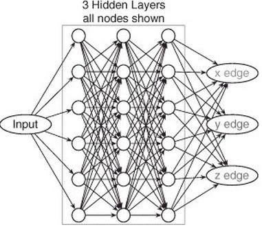
Our CN has an architecture with three hidden layers, each containing six feature maps. All filters in the CN are of size 5 × 5 × 5, but since CN contains four convolutions between input and output, a single output voxel is a function of a 17 × 17 × 17 voxel region of the input image.
Here is their diagram of their CN which I am still trying to fully understand:
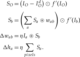
They give formulae for the CN itself: (eq 2.1)
As well as for the gradient backpropagation algorithm: (eq 2.2)
I haven’t so far made sense of these other than it seems you run eq 2.1 first, and then eq 2.2 in the opposite direction. Appendix B.1 describes the gradient backpropagation in more detail, but this is still going to take me some more time to decipher.
It sounds like the performance of their approach is quite good– they were able to correctly classify (does that mean cut vs. no cut?) 90% of edges, and that figure was about the same on the training vs. test sets, indicating the model didn’t get overfitted. From what I can tell they did not use either of the error measurements (warping error or Rand error) mentioned in the Jain et al article– instead they used precision-recall curves to measure the error of the affinity graph and splits and mergers to measure the error of the segmentation (Appendix C).
While all this is very interesting, the most shocking part of the whole article is this small factoid:
White et al. (1986) took over 10 years to complete the manual reconstruction of the entire nervous system of a nematode worm C. elegans, which contains only 302 neurons


