How PCR duplicates arise in next-generation sequencing

PCR duplicates are an everyday annoyance in sequencing.  You spend hundreds or thousands of dollars to get sequencing done, and after you get the reads back, you find that several percent, sometimes even 30% or 70% of your reads are identical copies of each other.  These are called PCR duplicates and most sequencing pipelines recommend removing them or at least marking them (Picard’s MarkDuplicates or samtools rmdup are two available tools).

Ever since I got into sequencing I wanted to know how these duplicates arise – what does it mean for a read to be a PCR duplicate and why do we ignore them?  I’ve Googled this over and over and never found a satisfying explanation.  So after hearing Shawn Levy give an excellent introduction to the biochemistry and technology of sequencing at the first day of the UAB sequencing course, I asked him how PCR duplicates arise in next-generation sequencing.  In this post I’ll explain the answer he gave me.

First, let’s put this in context of the basic steps of library prep and sequencing:

1. Shatter genomic DNA, e.g. with a sonicator.
2. Ligate adapters to both ends of the fragments.
3. PCR amplify the fragments with adapters
4. Create an oil-water emulsion of micrometer beads and DNA molecules (for Roche or Ion Torrent technologies) or spread DNA molecules across flowcells (for Illumina technology).  Goal is to get exactly one DNA molecule per bead or per flowcell lawn of primers.  This depends purely on probability, based on the concentration of DNA.
5. Use bridge PCR to amplify the single molecule on each bead or each lawn so that you can get a strong enough signal (whether light or pH) to detect.  Usually this requires several hundred or low thousands of molecules.
6. Sequence by synthesis of complementary strand: pyrosequencing  (Roche), reversible terminator chemistry (Illumina), or ion semiconductor (Ion Torrent).

PCR duplicates arise in step 3.  In step 3 you are intentionally creating multiple copies of each original genomic DNA molecule so that you have enough of them, therefore some amount of PCR duplication is inevitable.  PCR duplicates occur when two copies of the same original molecule get onto different beads or different primer lawns in a flowcell.  Ideally in step 3 you are amplifying only ~64-fold (Shawn Levy said he prefers to do no more than 6 rounds of PCR, hence 2⁶) and so the library still has high “complexity”, i.e. information entropy.  This will let you have the fraction of your final reads that are PCR duplicates can be as low as 4%.  Higher rates of PCR duplicates e.g. 30% arise when people have too little starting material such that greater amplification of the library is needed in step 3, or when people have too great a variance in fragment size, such that smaller fragments, which are easier to PCR amplify, end up over-represented.

This whole explanation depends upon the random assignment of molecules to beads, beads to molecules that occurs in step 4.  You can only generate interpretable reads if you have monoclonal beads or clusters by the time you get to step 5.  Polyclonal beads – where more than one distinct DNA molecule arrived in step 4 – always arise in sequencing, and sequencers have software for masking out and ignoring these picotiter wells or these clusters on a flowcell.  Similarly, software will ignore empty wells or empty clusters where no DNA molecule wound up.  Sometimes more than one copy of the same original molecule (say, 2 out of the 64 copies you made of each molecule) which each hybridize to a different bead, and so you’ll be reading the same DNA in two different wells/clusters – those are your PCR duplicates.  But the goal is to have the concentrations of DNA and of beads/lawns just right in step 4 such that it’s likely that the majority of beads/clusters will get exactly one DNA molecule, and very few unique DNA molecules will be represented more than once.

Does that make sense?  I had to sit down and work through the probability myself.  The random hybridization of DNA molecules to beads is kind of complicated: it’s like drawing different-colored balls from different bins and then dropping those balls into different bins.  As a simplifying assumption, let’s suppose all beads will end up monoclonal, and only ask the question of how many DNA molecules will end up represented 0, 1, 2… n times in the resulting reads.

Here’s some quick back-of-the-envelope: say your NGS technology requries 1μg of DNA as input (figure quoted here).  If, as Shawn Levy recommends, you’ve done 6 PCR cycles, then that means you must have started with 1μg/(2⁶) = 15.6 ng of DNA isolated from your sample.  Molecular weight of DNA averages around 660g/mol/bp, and let’s say your fragments average 200bp long, so you’ve got 15.6ng/(660e9ng/mol/bp*200bp)*(6.022e23molecules/mol) = ~7e10 unique molecules.  If you’re doing 20x whole genome sequencing with 100bp reads, you’ll want 20x*3e9b/100b = 600M reads.  Since we’re simplifying and assuming for now that all beads will be monoclonal, for now let’s assume 600M reads means 600M = 6e8 beads.

So far you’ve got 64 copies each of 7e10 unique molecules and you want to hybridize them to 6e8 beads.  The expected number of copies of each molecule represented in your reads will be 6e8/7e10 = .0085.  In order to figure out the PCR duplicate rate, it would be nice to know the fraction of the 7e10 unique molecules that will be represented 0, 1, 2, … n times in the output reads.  You could model this as a binomial distribution with p = 1/(7e10) and n = 6e8, but since the probability is very low and number of trials very high, this will be better modeled by the asymptotic limit of the binomial: the Poisson distribution.  The PDF of the Poisson distribution is given by λ^ke^-λ/k! where k = 0,1,2,…n is the number of copies of the molecule drawn, and the parameter lambda is equal to the expected number of copies of each molecule, which as I’ve said above is ~ .0085.

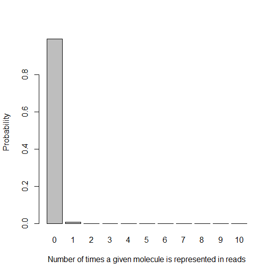
With these parameters, I generate in R a histogram of the probability of a given molecule being represented 0, 1, 2, etc. times:

x = seq(0,10,1)
xnames = as.character(x)
xlab = "Number of times a given molecule is represented in reads"
ylab = "Probability"
barplot(dpois(x,lambda=.0085),names.arg=xnames,xlab=xlab,ylab=ylab)

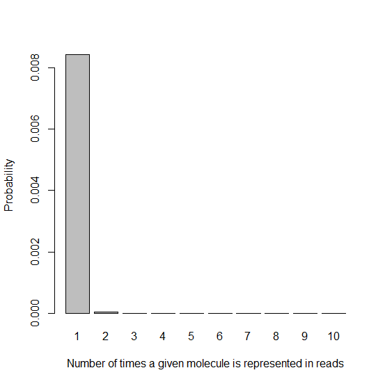
As you’d expect, since we have far more molecules than beads, most reads get represented 0 times.  That’s fine – we started with many copies of the genome extracted from many cells, and we’ll get plenty of coverage from the handful of reads that are represented.  The important thing from this histogram is the very high height of the “1″ bar  compared to all the ones that come after it, which is difficult to see in the above histogram because everything is dwarfed by the “0″ bar.  Let’s exclude that bar:

x1 = seq(1,10,1)
x1names = as.character(x1)
x1lab = "Number of times a given molecule is represented in reads"
ylab = "Probability"
barplot(dpois(x1,lambda=.0085),names.arg=x1names,xlab=x1lab,ylab=ylab)

This histogram looks really good: given that a DNA molecule is represented in a read at all (since we’ve filtered out the k=0 molecules), it’s overwhelmingly likely that it’s represented exactly once.  And luckily, even if it’s represented twice, that’s not two PCR duplicates, just one – we’ll still use one copy and throw the other out.  Therefore we can quantify the fraction of PCR duplicates with this expression:

sum(dpois(x1,lambda=.0085)/x1)/(1-dpois(0,lambda=.0085))

Just to explain: sum(dpois(x1,lambda=.0085)/x1) is just count(1)/1 + count(2)/2 … i.e. summing the number of unique reads, and dividing (1-dpois(0,lambda=.0085)) is just normalizing for the fraction of molecules that get sequenced at all.

The expression evaluates to .9979, so only 0.21% PCR duplicates.  The fact that this is different from Shawn Levy’s quoted figure of 4% under ideal conditions is due to some combination of (1) my back-of-the envelope numbers were off by a bit, and (2) even if you do everything right you’ll have some bias where by short length, low GC-content fragments are overrepresented, whereas I’ve assumed uniformly amplification of every starting molecule.

This model looks useful, so let’s continue with it.  Now suppose that instead of 7e10 unique molecules amplified 64-fold, you started with a smaller sample of just ~9e9 molecules and ran 9 PCR cycles, thus amplifying them 2⁹ = 512-fold.  Now the lambda parameter in your Poisson distribution has risen to 6e8/9e9 = 0.067.  You started with so few unique molecules that on expectation each one will be represented 0.067 times.

Plugging this into our expression:

sum(dpois(x1,lambda=.067)/x1)/(1-dpois(0,lambda=.067))

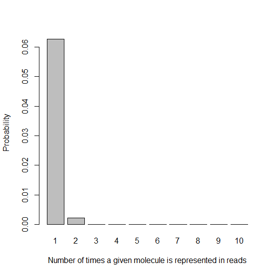
We get .983, so a 1.7% PCR duplicate rate, still small but much higher than before. It’s easy to see why this occurs by looking at the histogram:

barplot(dpois(x1,lambda=.067),names.arg=x1names,xlab=x1lab,ylab=ylab)

You can see that the bar for k=2 is subtly taller than it was in the histogram with lambda = .0085.  Due to our lower number of unique molecules to start with, more molecules are getting represented twice, meaning you get more reads that are PCR duplicates.

We can look at an even worse scenario: maybe you started with just 1e9 unique molecules and did 12 PCR cycles, thus 2¹² = 4096 copies of each molecule.  Now your Poisson lambda is 6e8/1e9 = 0.6.  Plugging that in we see:

sum(dpois(x1,lambda=.6)/x1)/(1-dpois(0,lambda=.6))

= .85, implying 15% of reads will be PCR duplicates. And this is even easier to see on the barplot –  the k=2, 3, 4 etc. bars are very visibly higher:

barplot(dpois(x1,lambda=.6),names.arg=x1names,xlab=x1lab,ylab=ylab)

This whole analysis, while simplified, illustrates at least two important points about this random bead-DNA selection step 4 which arise from the Poisson distribution:

• The lower your ratio of unique molecules to beads, the more PCR duplicates you will have, even before your ratio begins to approach 1.0, where PCR duplicates would be required in order to saturate the beads with DNA molecules.
• Even with 64 copies each of the unique molecules, PCR duplicates are very rare by pure chance.  Each unique molecule’s chance of getting represented even once (let alone twice) is small.