The math behind Spearman-Karber analysis
In the study of prions, endpoint titration (also known as endpoint dilution) is a bread-and-butter method for quantifying the number of prions in a sample. It’s used both in bioassay, where the quantity derived is called an “infectious unit” or “infectious dose”, and in RT-QuIC, where the quantity is called a “seeding unit”. Intuitively, the logic employed is obvious: if you can dilute a sample 10-8 and still cause disease in an animal, or a positive replicate in RT-QuIC, then there must have been 108 prions in the original undiluted sample. But though I’ve used this method several times and have read papers that used it hundreds of times, I recently realized that I actually had no understanding of what the greater mathematical reasoning behind this method is. In particular, how does one determine the standard error around one’s estimate of the median infectious dose (ID50) or median seeding dose (SD50), and how can one tell if two estimates from two different experiments are statistically different?
The formula most often used is attributed to Spearman and Kärber. But whatever book or paper those two individuals wrote, it is so old that not only does no one directly cite it, none of the references that people cite cite it either. Most of the papers I’ve seen cite one of the following two references:
- Dougherty RM. Animal virus titration techniques. In: Harris RJC, editor. Techniques in Experimental Virology. New York: Academic Press; 1964. pp. 183–186.
- Martin A. Hamilton, Rosemarie C. Russo, and Robert V. Thurston. Trimmed Spearman-Karber Method for Estimating Median Lethal Concentrations in Toxicity Bioassays. Environmental Science & Technology. 1977. doi: 10.1021/es60130a004. full text.
Both of which are themselves ancient, and neither of which actually contains anything by a Spearman or a Kärber in the references. But after tracking down copies of these two works I made an effort to wrap my mind around the math behind this analysis.
Suppose you’ve got these data from an RT-QuIC experiment:
Table 1
| x = log10(dilution) | n = number of replicates or animals | number positive | p = proportion positive |
|---|---|---|---|
| -1 | 4 | 4 | 1.0 |
| -2 | 4 | 4 | 1.0 |
| -3 | 4 | 4 | 1.0 |
| -4 | 4 | 4 | 1.0 |
| -5 | 4 | 4 | 1.0 |
| -6 | 4 | 4 | 1.0 |
| -7 | 4 | 4 | 1.0 |
| -8 | 4 | 3 | 0.75 |
| -9 | 4 | 1 | 0.25 |
| -10 | 4 | 0 | 0.0 |
In addition to the variables x, n, and p in the table above, we also define two more:
\[d := log_{10}(dilution\ factor)\] \[x_{p=1} := argmin_x (p_x = 1)\]In the example above, we are doing serial 10-fold dilutions, and log10(10) = 1, so d = 1. xp=1 is the most dilute value of x for which p=1, so here, -7. The log10(SD50) is traditionally defined as:
\[log_{10} {SD_{50}} := x_{p=1} + \frac {1}{2} d - d \sum {p}\]Perhaps for posterity, people continue to write the formula that way (see for instance [Wilham 2010]), but it’s kind of confusing. First, Σp doesn’t mean sum across all p; it’s explained offline that it means for all p from xp=1 out to the most dilute dilution tested. If you wanted to express that right in the formula, you might write:
\[log_{10} {SD_{50}} := x_{p=1} + \frac {1}{2} d - d \sum_{x_{p=1}}^{x_{min}} {p_x}\]Where xmin is the most dilute dilution.
But a second quibble is that it’s kind of non-intuitive how the terms of the formula make us backtrack away from the best estimate before coming back around again. Looking at the data, the best estimate of log10(SD50) is obviously going to be between -8 and -9. Unpacking the formula, we start with xp=1 = -7, and next we add ½d, which moves us further away, to -6.5. Then the last term is simply the sum of the value of p at -7 to -10, so 1.0 + .75 + .25 = 2. So our best estimate comes out to -8.5. Becuase xp=1 is defined as, well, the lowest x where p=1, and yet we add pxp=1 in the summation, we’re tautologically adding a 1d. Why do that? Instead, let’s make life easier and just define:
\[i := x_{p=1}\]So the formula becomes:
\[log_{10} {SD_{50}} := i + \frac {1}{2} d - d \sum_{i}^{x_{min}} {p_x}\]And then let’s rearrange a bit:
\[log_{10} {SD_{50}} := i - d( \frac {1}{2} + \sum_{i - d}^{x_{min}} {p_x} )\]So now, more intuitively, reading left to right, we start with -7, then subtract a half to get -7.5, then subtract (.75 + .25 + 0.0) to get -8.5, our estimate. Bear in mind that this value estimates to the log10 dilution at which 50% of replicates would be positive. Swap the sign on that estimate, and you have the log10 number of seeding units, in the original sample, per whatever volume you’re seeding. In RT-QuIC, wells are usually seeded with 2μL of a sample, so these data would imply that every 2μL of pure brain, or CSF, or whatever your original sample was, contains 108.5 seeding units. You might choose to express your estimate per mL or some other unit, so in this case, 500 × 108.5 = 5 × 1010.5 seeding units per mL.
As an aside, neither reference explains how exactly the above formula is derived, but from what I gather, it does not seem to rest on an assumption of any underlying distribution. For instance, you might think that the number of infectious units drawn up in a given aliquot from a large population would be approximated by the Poisson distribution, but here, no one even gets into that level of detail. The assumption seems to be just that your sample means p are simply estimates of some true population mean P at each dilution, and that the true P across your dilutions follow a symmetric S curve. And you are just trying to find the midpoint of the S curve.
So what about standard error? The formula is given as:
\[SE := \sqrt { d^2 \sum { \frac {p(1-p)}{n-1} } }\]In this case, you can feel free to just take the summation over all values of x, since the p(1-p) term will be 0 for any dilutions that gave 100% negative or 100% positive responses.
In the case of the data above, this works out to ((.75.25)/(4-1) + (.25.75)/(4-1))½ ≈ .353. Thus, your 95% confidence interval, which is ±1.96×SE, comes to -7.8 to -9.2. So the true value could reasonably be at the -8 or -9 dilution, but would be very unlikely to like at the -7 or -10 dilution.
That makes intuitive sense if you think about it. I do think the actual number in any given replicate should be pretty well modeled by a Poisson distribution. So when you’re right at the endpoint, where the mean number of prions per replicate is by definition 1, the probability of any given replicate receiving zero prions is given by (in R code) dpois(x=0,lambda=1) = 37% (1/e, that magic number again).
But if you’re doing 10-fold dilutions, then at the next stronger dilution, the mean number of prions per replicate rises to 10. That makes it exceptionally unlikely that you’ll get even a single negative replicate. For any given replicate, dpois(x=0,lambda=10) = 4.5e-5, and so for, say, four replicates, the probability is (1-dpois(x=0,lambda=10))^4 = 99.98% that all four will be positive. Similarly, one dilution down from the endpoint, your mean numebr of prions per replicate is 0.1, so it’s fairly likely — dpois(x=0,lambda=.1)^4 = 67% — that all four replicates will be negative. Thus, it makes intuitive sense that the 95% confidence interval doesn’t extend further than 1 dilution in either direction from the best estimate.
Nevertheless, one may occasionally see data where p is non-monotonic. For instance, say you collected these data:
Table 2
| x | n | n pos | p |
|---|---|---|---|
| -5 | 4 | 4 | 1.0 |
| -6 | 4 | 2 | 0.5 |
| -7 | 4 | 0 | 0.0 |
| -8 | 4 | 1 | 0.25 |
| -9 | 4 | 0 | 0.0 |
Intuitively, that one irritating positive replicate at -8 would seem to drag our best estimate of SD50 upward, and also bump the variance on the estimate up. You might think that because we see that one positive replicate at -8, the estimate should be higher, and its standard error larger, than would be the case if the values of p for x=-7 and x=-8 in Table 2 were swapped. Yet if you look at the formulae for the best estimate of SD50 and for the standard error, neither one of them ever multiplies a value of x by a value of p. In other words, once you choose that xp=1 value to start from, all p above that value are treated equivalently. So, surprisingly, neither the estimate nor the standard error would change if, in the above table, I swapped the values of p for x = -7 and x = -8.
Accordingly, both Dougherty and Hamilton state that the standard error formula (though curiously, not the best estimate formula) require that p be non-increasing. Each provides a formula for how to “smooth” the data if this condition is not met. Hamilton’s is simpler — just average adjacent values until they’re non-increasing. In other words, in R:
smooth_p = function(p) {
    if (length(p)<2) {
        return (p)
    }
    while (any(cummin(p) != p)) { # while p is non-monotonic
        for (i in 2:length(p)) { # starting from the second dilution and going up,
            if (p[i] > p[i-1]) { # if the current one has higher p than the last one...
                # select all dilutions below the current one that have lower p...
                indices_to_average = c(which(1:length(p) < i & p < p[i]), i)
                # and average them all together with the current value.
                p[indices_to_average] = mean(p[indices_to_average])
            }
        }
    }
    return (p)
}
Hamilton also offers another optional tweak, which is the trimmed Spearman-Kärber estimator, in which basically you pick some tolerance value within which you’ll round p up or down to 1 or 0. For instance, you can just choose to set all p < 10% to 0, and all p > 90% to 1. The logic behind this is apparently that you imagine your population (fish, in his case) vary in their intrinsic susceptibility to the thing being measured (a toxin, in his case), and you want to base your estimate more on the average fish and less on the handful of fish that are exceptionally susceptible or exceptionally resistant to the toxin.
I’d argue that this particular logic makes more sense in a genetically heterogeneous population. In inbred mice with the same Prnp genotype, prion infection is like clockwork. And since the trimming is an added mathematical complication, I think I’ll stick with the regular-old estimator.
All that being said, here’s an R implementation of the formulae above, in R:
spearman_karber = function(x, n, p) {
    d = min(abs(diff(x))) # find d, the difference between dilutions
    if (any(abs(diff(x)) - d > .001)) { # .001 provides some numeric tolerance
        stop("x are not uniformly distributed\n")
    }
    nd = length(x) # number of dilutions
    p = smooth_p(p) # smooth the proportion positive to be non-increasing
    i = max(which(p==1)) # find the weakest dilution with all positive responses
    sd50 = x[i] - d*(1/2 + sum(p[(i+1):nd])) # calculate log10(sd50)
    estimate = -sd50 # estimate of seeds in original sample is opposite of the sd50
    se = sqrt(d^2 * sum(p*(1-p)/(n-1))) # calculate standard error
    return_value = list(estimate=estimate, se=se)
    return (return_value)
}
# test using data from Table 1
x = -1:-10
n = rep(4,10)
p = c(rep(1,7),.75,.25,0)
spearman_karber(x,n,p)
# test using data from Table 2
x = -5:-9
n = rep(4,5)
p = c(1, .5, 0, .25, 0)
spearman_karber(x,n,p)
Armed with the understanding of these formulae, we can now ask how to maximize power in our experiments. As far as I can tell, absolutely everyone does log10 dilutions absolutely all of the time. Is that the right thing to do? Or, all else being equal, would you get a tighter and more accurate estimate of the true number of prion seeds by doing a smaller number of replicates on each of a tighter series of dilutions, or a larger number of replicates on more disperse series of dilutions?
I have wondered about these sorts of questions ever since learning about how the 1000 Genomes project originally decided to do low-coverage (4x) whole-genome sequencing. Evidently this bit of skulduggery was one of Richard Durbin’s biggest contributions to the project: he did the math to show that for the project’s goals of discovering genetic variation in the population and determining the phase of variants relative to each other, for a given sequencing cost, power was maximized by sequencing many individuals lightly. To me, it is non-intuitive that you’d be better off having loads of genotype calls, no single one of which you can trust very much, than having a smaller number of high quality, high confidence calls.
To try to figure out whether similar logic applies to endpoint dilutions, I cooked up this simulation. Here, I am randomly generating data on positive replicates on the assumption that the true P is determined by the Poisson distribution as discussed above.
simulate_sk = function (fold, true_seeds=NA, xmax=-1, xmin=-10, n_avail=100, n_iter=1) {
    d = log10(fold) # user gives a fold dilution, i.e. 10, and this determines d
    x = seq(xmax,xmin,-d) # figure out what the dilution values will be
    n = rep(floor(n_avail / length(x)), length(x)) # evenly divide up the available replicates between dilutions
    p = rep(as.numeric(NA), length(x)) # create an empty p vector
    result = data.frame(estimate=numeric(n_iter), se=numeric(n_iter))
    for (k in 1:n_iter) { # for every randomized iteration
        # if true_seeds is NA, randomize it; otherwise use a user-specified value
        if (is.na(true_seeds)) {
            m = -runif(n=1, min=xmin+2, max=xmax-2)
        } else {
            m = true_seeds
        }
        for (j in 1:length(x)) { # using Poisson distribution, simulate proportion positive at each dilution
            p[j] = mean(rpois(n[j],lambda=10^(m + x[j])) > 0)
        }
        sk = spearman_karber(x,n,p)
        result$diff[k] = sk$estimate - m # positive means we overestimated, negative means underestimated
        result$se[k] = sk$se
    }
    return (result)
}

folds = c(2, exp(1), 10^.5, 10, 10^1.5, 10^2, 10^2.5, 10^3) # dilution schemata to test
nf = length(folds)
result = data.frame(fold=folds, diff=numeric(m), se=numeric(m))
for (i in 1:nf) {
    res = simulate_sk(fold=result$fold[i], n_iter=10000)
    result$diff[i] = mean(res$diff, na.rm=TRUE) # remove NA because occasionally you'll happen to get an inconclusive result
    result$se[i] = mean(res$se, na.rm=TRUE)
}
The result? First off, in this simulation, the Spearman-Kärber estimator is biased. It’s biased upward by about .25, so in other words, if your true number of prion seeds is 6.25 log10 units, the estimator will on average tell you it’s 6.5 log10 units. My guess is that this apparent bias arises from the fact that I’m assuming the underlying probabilities are Poisson-distributed, which means an asymmetric S-curve, whereas the Spearman-Kärber assumes symmetry. Who’s right? I don’t know. But in terms of standard error, perhaps surprisingly, it makes essentially no difference what dilution scheme you use. If you have 10 logs of range you want to cover, and 100 wells to use, it doesn’t matter if you do 10 replicates at ten 10-fold dilutions, or 20 replicates at five 100-fold dilutions. The standard errors appear to be very slightly smaller around the 100-fold range than the 10-fold range, but I’m not certain this is even real.
Here are what the data look like for the above simulation, with n=10,000 iterations on each simulated condition.
png('~/d/j/cureffi/media/2015/09/spearman-karber-simulation.png',width=800,height=500,res=100)
par(mar=c(6,4,2,2))
plot(NA, NA, xlim=c(0,3.25), ylim=c(-2,2), axes=FALSE, xlab='', ylab='',xaxs='i',yaxs='i')
abline(h=0,lwd=1,lty=3)
points(log10(result$fold), result$diff, pch=19, cex=1.5, col='#8912BA')
segments(x0=log10(result$fold), y0=result$diff - 1.96*result$se, y1=result$diff + 1.96*result$se, lwd=5, col='#8912BA')
axis(side=1, at=log10(folds), labels=c('2-fold','natural log','half-log','10-fold','1.5 log','100-fold','2.5 log', '1000-fold'), las=2)
abline(h=-2, lwd=2)
axis(side=2, at=-2:2, labels=-2:2)
mtext(side=1, text='dilution scheme', line=4)
mtext(side=2, text='normalized log10 estimate', line=3)
dev.off()
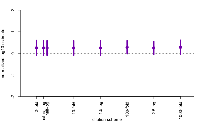
The points represent the mean difference between the estimate and the true SD50 value being simulated, so the fact that they’re all above 0 reflects the bias discussed above. The error bars represent the average 95% confidence interval around the estimate, which is ±1.96 SE. If you squint, the 95%CI is just slightly tighter for 100-fold and 2.5 log (i.e. 316-fold) dilutions than for the others, but the difference is trivial.
So if you’ve been doing 10-fold dilutions your whole life, carry on. No harm in following convention, particularly since, after all, your species has 10 fingers.

About Eric Vallabh Minikel
Eric Vallabh Minikel is on a lifelong quest to prevent prion disease. He is a scientist based at the Broad Institute of MIT and Harvard.