Adiga on Bright Field Microscopy
This post is a review of this article I just read [full text]:
Adiga U, Taylor D, Bell B, Ponomareva L, Kanzlemar S, Kramer R, Saldhana R, Nelson S, Lamkin TJ. 2012. Automated Analysis and Classification of Infected Macrophages Using Bright-Field Amplitude Contrast Data. Journal of Biomolecular Screening 17(3) 401–408. DOI: 10.1177/1087057111426902
Adiga et al have an approach that’s elegant, effective and more in line with how I’ve been thinking than any of the other image segmentation papers I’ve been reading lately.
They are working with bright field microscopy images. This is very simple: you shine a light through the samples and measure the light transmitted. They literally used an LED flashlight for this. This is distinct from light microscopy (e.g. with H&E) where you shine a light _on_ the samples and measure light reflected, or immunohistochemistry / fluorescence microscopy where you tag some type of molecule with fluorescent stains and measure light emitted. They are doing this in cell culture; I don’t know of any examples of doing this on in vivo samples or whether it would work given the necessary thickness of in vivo sections. So it may be that not all of this is relevant to the in vivo samples I’ve been working with, but much of the methodology is still relevant, and it could all be relevant to the broader goal of prion therapeutic assay development.
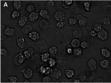
The trouble with bright field microscopy, the authors point out, is that cells are mostly transparent and organelles are too small to make out given the light wavelength. So what you end up with is a very low contrast image where the cells are distinguishable from the background mostly just by their different texture. To wit:

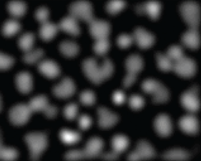
So yeah, not quite as obvious how to segment this as a fluorescent image with a black background and glow-in-the-dark cells. But my philosophy is if I can see the cells, a computer can see the cells too. You just need to think about what makes them visible to you, and write a program that looks for the same things. These authors seem to have the same instinct. Because texture is at issue, they start with a simple local texture detector. It’s amazingly simple: the value of each pixel in the new image is set to the square root of the sum of the squared difference in intensity between the pixels immediately to its left and right, and the pixels immediately to its top and bottom. This transforms an image where cells are highly textured and the background smooth to an image where cells are bright and the background dark. Then they blur it with a Gaussian filter to get rid of some of the residual texture so it doesn’t interfere with the visibility of what are generally bright, round cells. Next they multiply the blurred image by the original image (pixel-wise) and linearly rescale intensity to take up the full range. Finally they generate “a very low-frequency version of the contrast-enhanced image” as a reconstructed background image and subtract it from their contrast-enhanced image to reduce background texture. (I’m not sure I understand this step), and then smooth the resulting image again. That gets them this (Figure 2C):
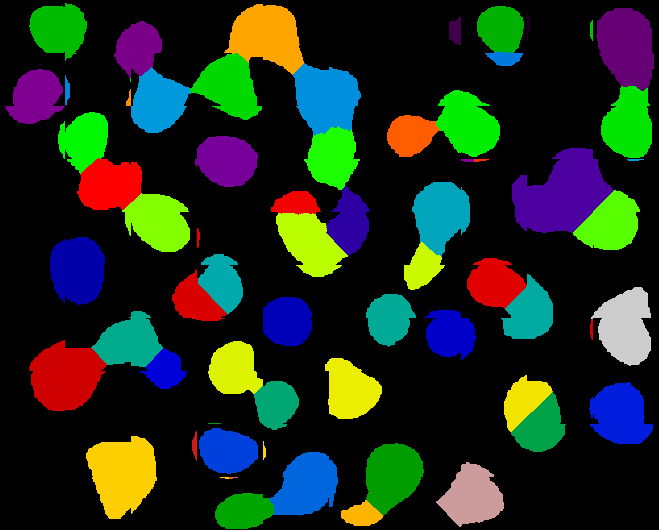
That’s all the pre-processing. Then their segmentation step is minimum error thresholding followed by fill-holes and then watershed to separate touching cells. But as you can see from their Figure 2C, the pre-processing is so good you could probably just feed this image into CellProfiler or other existing software and get pretty good results without even implementing any of your own logic. In fact, I screen captured their Figure 2C image and spent just a few minutes playing with it in CP and was able to do this well:
Which compares reasonably well to what the authors got (left to right, input image after the authors’ pre-processing, my segmentation with CP, and the authors’ segmentation using their approach).
My cell count is 66, while their (automated) count is 52 according to Fig 2F, but I think theirs is probably erring on the low side (you can see a couple of cells that their algorithm clearly missed). Also CP seems to have some wierd bug where it is finding a few tiny slivers of objects around the actual cells. Not sure what that’s all about. Anyway a bit more time with CP could probably improve on these results I got. My IdentifyPrimaryObjects settings were:
IdentifyPrimaryObjects:[module_num:3|svn_version:\'10826\'|variable_revision_number:8|show_window:True|notes:\x5B\x5D]
    Select the input image:inputgray
    Name the primary objects to be identified:cells
    Typical diameter of objects, in pixel units (Min,Max):10,40
    Discard objects outside the diameter range?:No
    Try to merge too small objects with nearby larger objects?:No
    Discard objects touching the border of the image?:Yes
    Select the thresholding method:RobustBackground Adaptive
    Threshold correction factor:.5
    Lower and upper bounds on threshold:0.000000,1.000000
    Approximate fraction of image covered by objects?:0.01
    Method to distinguish clumped objects:Shape
    Method to draw dividing lines between clumped objects:Shape
    Size of smoothing filter:10
    Suppress local maxima that are closer than this minimum allowed distance:7
    Speed up by using lower-resolution image to find local maxima?:Yes
    Name the outline image:PrimaryOutlines
    Fill holes in identified objects?:Yes
    Automatically calculate size of smoothing filter?:Yes
    Automatically calculate minimum allowed distance between local maxima?:Yes
    Manual threshold:0.3
    Select binary image:None
    Retain outlines of the identified objects?:No
    Automatically calculate the threshold using the Otsu method?:Yes
    Enter Laplacian of Gaussian threshold:0.5
    Two-class or three-class thresholding?:Two classes
    Minimize the weighted variance or the entropy?:Weighted variance
    Assign pixels in the middle intensity class to the foreground or the background?:Foreground
    Automatically calculate the size of objects for the Laplacian of Gaussian filter?:Yes
    Enter LoG filter diameter:5
    Handling of objects if excessive number of objects identified:Continue
    Maximum number of objects:500
    Select the measurement to threshold with:None
They also do fluorescence microscopy on the same images and compare results. First off, by the comparison of images you can see that the fluorescence is just going to miss some cells because they did not stain well even though they’re very visible in the bright field images. Also the fluorescence staining sometimes only gets part of the cell and isn’t uniform so you could miss a part of the cell. They compare their automated segmentation on the bright field and fluorescent images to a manual ground truth using yet another error metric, symmetric difference. This is the number of pixels considered foreground in one segmentation but not the other, divided by the number of pixels in the ground truth segmentation. So in this metric, higher numbers are worse. Their algorithm averages 11% error on bright field and 18% on fluorescent images. Just looking at their segmentation (on bright field images) you can also just see that it’s quite good.
Another cool thing about this paper is they then do high-content feature analysis to try to distinguish infected from uninfected cells (macrophages infected with Franciscella tularensis), with some success. This is the first place I have actually seen a list of the types of features one can use in this type of analysis:
We have calculated more than 1000 features for each cell image. These features include basic size and shape descriptors, multiscale features, invariant moment features, statistical texture features, Laws texture features (statistical texture features of Laws texture images), differential features of the intensity surface (features of local gradient magnitude, local gradient orientation, Laplacian, isophote, flowline, brightness, shape index, etc.), frequency domain features, histogram features, distribution features (radial, angular, etc. of intensity distribution, gradient magnitude distribution), local binary pattern image features, local contrast pattern image features, cell boundary features, edge features, and other heuristic features such as spottiness, distance between histograms of pixel patches and between concentric circular areas within the cell, gray class distance, heuristic and problem-specific features, and so on. Features were calculated for each cell and normalized to have a value between 0.0 and 1.0.
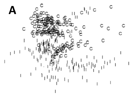
Another thing in this paper that I need to learn more about is how they produced the “two-dimensional multidimensional scaling (MDS) ordination plot” in Figure 4. They have 1000+ features on their samples, so you can think of these samples in a 1000+dimensional feature space, and each sample has a Euclidean distance from other samples that could be calculated as the square root of the sum of squared differences in every dimension. But these folks have some way of projecting that 1000+dimensional scatterplot onto a 2D plane. Obviously a lot of information is lost here but the images still manage to demonstrate that their features have classification value, since the control and infected cells only overlap a little bit in their distributions:
Multidimensional scaling does have its own article on Wikipedia but the section on how you actually boil down the n-dimensional space to a 2-dimensional figure has been hilariously labeled void for vagueness:
The dimensions must be labelled by the researcher. This requires subjective judgment and is often very challenging.[vague] The results must be interpreted (see perceptual mapping).[vague]
Borgatti offers a better explanation of the process, and it seems to be basically an iterative algorithm that seeks to minimize stress, where stress is a function of the sum of the differences between each pair of points’ true n-dimensional distance and mapped 2-dimensional distance.
A final note: the authors state that their C# .NET implementation of all this will be made available on request.


