Tips for dealing with NHGRI GWAS catalog data
Over the last few years, the U.S. National Human Genome Research Institute has made an effort to compile all the results of published genome-wide association studies into one big table, the GWAS catalog. This is an awesome dataset, with 9,977 trait-associated SNPs as of this writing, and has already proven to be a useful public resource enabling other research – for instance, Nicolae 2010‘s finding that GWA hits are enriched for eQTLs.
The data are a bit tricky to work with. Here’s what I’ve figured out.
Use this link to download the latest version of the catalog in tab-delimited txt form. Once you’ve downloaded it, you might want to read it into R. Two issues: (1) it contains special characters with HTML escapes such as ç, which will a default read.table statement in R will interpret as comments/quotes thus ending a line and giving you errors like line 2 did not have 34 elements, and (2) R will convert scientifically notated p values into factors, making it difficult to recast them to numeric later. What you need is this line of R code:
gwahits = data.frame(read.table('gwascatalog.txt',header=TRUE,sep='\t',quote="",comment.char="",as.is=TRUE))
Once you get to working with the data you’ll notice that many GWA hits are duplicated – i.e. the same SNP has been found associated with the same (or different) traits in different studies, so not all rows are unique:
> length(paste(gwahits$Chr_id,gwahits$Chr_pos))
[1] 9977
> length(unique(paste(gwahits$Chr_id,gwahits$Chr_pos)))
[1] 7912
You’ll also notice the data are non-relational, which is probably my biggest complaint about this (and every) bioinformatics dataset. For instance, multi-SNP haplotype GWA hits are reported as a single row with comma-separated values such as rs897200, rs7572482, rs7574070 and some other SNPs (that impact multiple genes?) are reported with semicolon-separated values such as PBX2;GPSM3. If you’re not already with me on the importance of the relational data model, just try to generate some descriptive statistics that include these rows – for instance, find the total number of GWA hits and minimum p value for each gene. You’ll probably end up needing to write your own Python script to parse the multiple values into separate rows.
Chromosomal coordinates aren’t reported for most of these complex rows (i.e. Chr_id and Chr_pos are NA), which makes it hard to do any BED-style operations. For instance, I wanted to intersect the GWA hits with a BED file of exons from the UCSC Table Browser in order to see how many GWA hits were exonic. To create a BED file for this, I had to subset just the unique non-NA rows:
gwabed = data.frame(gwahits$Chr_id,gwahits$Chr_pos,gwahits$Chr_pos)
gwabed = unique(gwabed[!is.na(gwabed$gwahits.Chr_pos),])
write.table(gwabed,file="gwahits.bed",eol="\n",row.names=FALSE,col.names=FALSE,sep="\t")
And then I used intersectBed -u via bash (add ‘chr’ to match UCSC’s hg19 formatting):
sed -i 's/^/chr/' gwahits.bed
intersectBed -a gwahits.bed -b UCSC_knownGene_exons -u > gwahits_exonic.bed
intersectBed -a gwahits.bed -b UCSC_knownGenes_WholeGene -u > gwahits_genic.bed
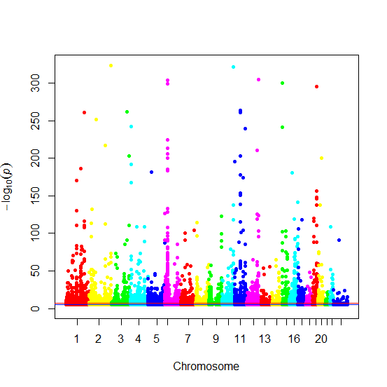
I also thought it would be interesting to make a Manhattan plot of the GWA hits. Normally you make Manhattan plots of sets of SNPs from unbiased association studies, so most SNPs are not significant – here we have a list of SNPs that are selected to all be significant. I used Stephen Turner’s awesome Manhattan plot code as follows:
source("http://dl.dropbox.com/u/66281/0_Permanent/qqman.r")
P = as.numeric(gwahits$p.Value)
CHR = gwahits$Chr_id
BP = as.integer(gwahits$Chr_pos)
gwa2 = unique(data.frame(CHR,BP,P))
manhattan(gwa2,colors=rainbow(6))
Producing this plot:
Note the magnitude of the log scale on the y-axis. I was surprised that, even though these are all trait-associated SNPs (and I selected for unique SNPs), you still see the characteristic pattern from which Manhattan plots get their name: the peaks of association form skyscrapers. I suppose that the accumulation of many associated SNPs clustered closely together reflects the fact that dozens of mutations in one important gene (or group of genes) could all be associated with traits related to that gene. For instance I note that the huge dense spike on Chromosome 6 (in purple) appears to correspond to the HLA, the site of a dense cluster of immune system genes and ground zero for autoimmune disease risk factors.

