Slope or correlation, not variance explained, allow estimation of heritability
In an earlier post on how to calculate heritability, two of the models I discussed rely on correlating the phenotypes of related individuals: sib-sib correlation and parent-offspring regression. In each case, you can compare two individuals who are expected to share 50% of their genome, and so double the correlation of their phenotypes provides an upper limit on additive heritability of that phenotype. (It’s an upper limit, not an estimate, because phenotypic similarity could be due partly to genetics and partly to shared environment).
However until now I’ve been confused about exactly what number is meant by the “correlation” of their phenotypes. I learned about parent-offspring regression from a recent review [Visscher 2008] which says that the slope of the regression line is what is important. For one parent – one offspring regression, you take 2x the slope, and for midparent – offspring regression, you take 1x the slope.
After I read this I wondered, why the slope and not the variance explained? Suppose I do a single parent-offspring linear regression and I get a slope of 0.4 (implying h2 ≤ 80%) but an R2 of only .12. Couldn’t you argue that if the parent’s phenotype only explains 12% of the variance in the child’s phenotype, then the trait can’t be more than 24% heritable?
To convince myself of which interpretation was correct, I had to do some experiments in R, which I’ll share in a moment.
But first, I also had to refresh myself on how the Pearson’s correlation coefficient (denoted r, rho or ρ) relates to linear regression. tl;dr: the Pearson’s correlation r is the square root of the unadjusted R2 (variance explained) from a linear regression. In other words, r and R are the same thing. If you need convincing, just make up any old dataset in R and check that the two are equal:
setseed(9876) # set a random seed so you get the same answer I do
series1 = seq(1,100,1) # make up some data
series2 = series1 + rnorm(n=100,m=0,sd=10) # make up some correlated data
m = lm(series2~series1) # linear regression
unadj.r.sq = summary(m)$r.squared # extract unadj R^2 from a linear model
correl = cor.test(series1,series2) # Pearson's correlation
r = as.numeric(correl$estimate) # extract r from cor.test result
sqrt(unadj.r.sq)
#[1] 0.9385556
r
#[1] 0.9385556
Moving on, my goal is to figure out whether the slope or the variance explained is the figure that relates to heritability. To do this, I simulated phenotypes for a series of 1000 made-up siblings:
# make up a bunch of random vectors
set.seed(9876)
a = rnorm(n=1000,m=0,sd=1)
b = rnorm(n=1000,m=0,sd=1)
c = rnorm(n=1000,m=0,sd=1)
# create a series of sib pairs for which a common factor (a) ought to explain ~50% of variance in "phenotype"
sib1 = a+b
sib2 = a+c
correl = cor.test(sib1,sib2)
r = round(as.numeric(correl$estimate),2)
m = lm(sib2~sib1)
slope = round(summary(m)$coefficients[2,1],2)
adj.rsq = round(summary(m)$adj.r.squared,2)
plot(sib1,sib2,pch=19,main="made up sib correlation",sub=paste("slope = ",slope," r = ",r," adj R^2=",adj.rsq,sep=""))
abline(m,col="red")
The idea is, there are 1000 pairs of siblings, so every index in the sib1 and sib2 vectors represents a pair, i.e. for all i, sib1[i] is the sibling of sib2[i]. These vectors hold the phenotypes of the two siblings. A common factor a contributes about half of the phenotype for each of them. Because the sibs share half their phenotype and share on average half their genome, this corresponds to a trait that could be up to 100% heritable (or it could all be shared environment effect). When you run the above code, you get this:
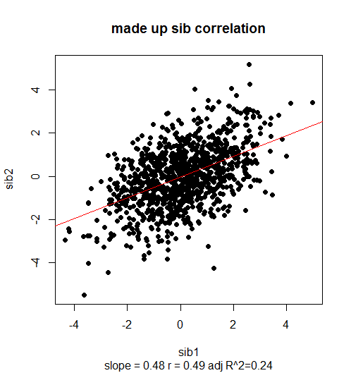
Since I made up the data, I know that the effect of a (representing half the additive genetic effect plus all the childhood shared environmental effect) should explain ~50% of the phenotype. The slope reflects this (.48 ≈ .50) and the variance explained (.24) does not. If you double the slope 2*.48 = .96 you get a reasonable estimate of the “true” heritability (~100%).
Or let’s do another example, in which the heritability should be only ~50%. Here I set the standard deviation of e and f (representing stochastic or non-shared environmental factors), to 1.7 (≈√3) so that d (the shared genetic factor), should only account for 25% of overall phenotypic variance.
# an example where the trait should be only ~50% heritable
set.seed(2222)
d = rnorm(n=1000,m=0,sd=1)
e = rnorm(n=1000,m=0,sd=1.7) # 1.7 ~ sqrt(3)
f = rnorm(n=1000,m=0,sd=1.7)
var(d)
#[1] 1.006501
var(e)
#[1] 3.038408
var(d)/var(c(sib1,sib2))
#[1] 0.2578496 # this is 1/2 of the "true" heritability
# now try to measure heritability by regression
sib1 = d+e
sib2 = d+f
correl = cor.test(sib1,sib2)
r = round(as.numeric(correl$estimate),2)
m = lm(sib2~sib1)
slope = round(summary(m)$coefficients[2,1],2)
adj.rsq = round(summary(m)$adj.r.squared,2)
plot(sib1,sib2,pch=19,main="another made up sib correlation",sub=paste("slope = ",slope," r = ",r," adj R^2=",adj.rsq,sep=""))
abline(m,col="red")
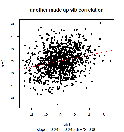
Again, 2*slope = .48 is pretty close to a correct heritability estimate (actually, according to 2*var(d)/var(c(sib1,sib2)) the true heritability ended up being ~51%). The R2 is miniscule, at .06.
So it appears to be 2*slope, not 2*(variance explained), that estimates the upper limit on heritability. Again, it’s an upper limit because the “shared” factors I spiked in (a and then d) could represent genetic or shared environmental factors. Indeed, as the collective genius of Wikipedia has put it:
sibling phenotypic correlation is an index of familiarity – the sum of half the additive genetic variance plus full effect of the common environment
But the use of the term “correlation” in this quote alludes to a fact you’ve probably noticed in both of the above examples: slope ≈ r.
Of course, there’s no rule that says r has to equal slope. By definition, Pearson’s correlation does not tell you anything about the steepness of slope (though its sign tells you direction of slope), as is beautifully illustrated in this Wikimedia Commons graphic:

Or if that doesn’t convince you, just make up some data in R to convince yourself:
x = seq(1,100,1)
y = x^2
r = as.numeric(cor.test(x,y)$estimate)
r
# 0.9688545
slope = summary(lm(y~x))$coefficients[2,1]
slope
# [1] 101
That said, it seems that r and slope are likely to be pretty close in any plausible model of a real genetic relationship. After all, for what earthly biological reason would one sibling’s phenotype ever be the square of the other’s? Especially when you consider there is usually no logical ordering to sib pairs (it’s random which member of any pair ends up plotted on which axis), you’re just unlikely to get a really steep slope with a really small r, or a really tight fit (large r) for a slight slope. They can vary a bit, but I can’t think of a good reason why the two quantities should be hugely different, so if I ever find that slope and r are wildly different, I’ll consider that a cue to do double check my data and my analysis.
The observation that r and slope are likely to be pretty similar may resolve a confusion I’ve had. The literature on twin studies [ex. Deary 2006 (ft); see also the above quote and Falconer's formula] and sib-sib correlation tends to refer to the “correlation” (presumably r) of the two siblings, while the literature on parent-offspring regression refers to the “slope” [Visscher 2008]. Perhaps this discrepancy owes simply to the fact that these quantities are very likely to be quite close in any real genetic dataset. If anyone can think of a reason why r is more correct for sibs and slope is more correct for parent-offspring, leave me a comment.

About Eric Vallabh Minikel
Eric Vallabh Minikel is on a lifelong quest to prevent prion disease. He is a scientist based at the Broad Institute of MIT and Harvard.