Analytical solutions for a model of prion protein degradation
introduction
A few months ago I blogged a numerical simulation of prion protein degradation. Now, at Sina Ghaemmaghami‘s suggestion, I’m returning to this issue to figure out an analytical solution.
Here’s a bit more background for math people who aren’t biologists reading this post. Prion diseases are caused by a normal protein called cellular prion protein (PrPC) misfolding into a diseased conformation called scrapie prion protein (PrPSc). In some anti-prion drug discovery screens, people take prion-infected cells and screen a whole library of tens of thousands of chemical compounds to look for compounds that will reduce the amount of PrPSc the cells accumulate. If your library has a compound that directly reduces PrPSc, you’re pretty likely to see that effect.
But what if there’s a compound whose mechanism is way far upstream? Remember that DNA → RNA → protein and (in this case), healthy protein → diseased protein. So for instance, what if a compound inhibits a transcription factor, preventing the prion protein gene’s DNA from being transcribed into RNA? In this case, the pre-existing messenger RNA (mRNA) will first need to decay with a certain half-life, and then as the level of mRNA gradually reduces, the amount of PrPC translated form that mRNA will gradually reduce, and then finally the amount of PrPSc converted from PrPC will gradually reduce. So switching off the supply of mRNA could take days to percolate through the system and show you an appreciable reduction in PrPSc. How many days? That’s what this post seeks to answer.
acknowledgements
When I set out to do this, it had been over a decade since I’d solved a differential equation. Thanks to Adam Bliss for a lot of help figuring out how to go about doing all this.
assumptions
I’ll assume that the degradation of PrP mRNA, PrPC and PrPSc is first-order, so they follow the standard rules of exponential decay. This is also what others have assumed and it’s pretty well-supported by experimental evidence [Ghaemmaghami 2007 + supplement].
The decay parameters of mRNA, PrPC and PrPSc will be denoted respectively by λ, μ and ν. I’ll assume the production rate of PrP mRNA is a constant denoted r. The production rate of PrPC is a constant a times the amount of mRNA present. The production rate of PrPSc is a constant β times the amount of PrPC present*. The quantities of PrP mRNA, PrPC and PrPSc as a function of time will be denoted by R(t), S(t) and T(t) respectively. The rates of change in these variables are then described in a system of differential equations:
} = r - \lambda\text{R(t)}")
} = \alpha\text{R(t)} - \mu\text{S(t)}")
} = \beta\text{S(t)} - \nu\text{T(t)}")
*I’ve assumed that the rate of PrPSc production is proportional to the amount of PrPC available as substrate but does not depend on the amount of PrPSc available to do the converting. This is surely a controversial assumption, as prion conversion requires PrPSc-PrPC binding. I’ll return to this subject in detail in an upcoming post. For now, I will stick to the assumption that the PrPSc formation rate is independent of [PrPSc], as I assumed in my original numerical simulations.
Finally, I’ll also assume we begin at steady state at t = 0 and will define the initial steady state quantities as:
")
")
")
For simplicity, when I plot later I’ll assume that all of those quantities are equal to 1.
Based on the literature reviewed in my original post the half-lives of mRNA, PrPC and PrPSc are about 7h, 5h and 30h, so I will define the constants λ0, μ0, and ν0 to be ln(2)/7 = .099h-1, ln(2)/5 = .14h-1, and ln(2)/30 = .023h-1 respectively. I will consider these as constants while I will use the symbols λ, μ, and ν to denote variables which can be modified by chemical compounds to perturb the cell from its initial steady state.
derivation
In my previous post I considered six possible mechanisms by which small molecules could reduce PrPSc accumulation. They might inhibit transcription (reducing r), promote mRNA degradation (increasing λ), inhibiting translation (reducing α), promoting PrPC degradation (increasing μ), inhibiting conversion (reducing β) or promoting PrPSc degradation (increasing ν).
First, let’s characterize the initial steady state at t = 0, before the cell has been perturbed by any chemicals. Since I’m going to treat r, α and β as variables that can be perturbed, I’ll need to define the constants r0, α0 and β0 to be the initial, unperturbed values of these variables. At t = 0,
 = 0 = r_0 - \lambda_0 R(0)")

 = 0 = \alpha_0 R(0) - \mu_0 S(0)")

 = 0 = \beta_0 S(0) - \nu_0 T(0)")

From these equations you can also probably guess a more general fact about the steady state values of all of these variables. For example, if I cut transcription by ½ or if I double the rate of mRNA degradation then I’ll wind up with half as much mRNA, and therefore half as much PrPC and half as much PrPSc as before.
My goal here is to see how quickly the system will advance toward that new steady state if we start from the initial steady state I’ve defined above. In other words, I need to obtain expressions for R(t), S(t) and T(t). Let’s start with R(t). I can get that by solving this differential equation:
 = r - \lambda R(t)")
Which I’ll do by guess-and-check. I’ll guess that R(t) has the form A + Be-λt. Let’s try it out:
 = A + Be^{-\lambda t}")
 = r - \lambda (A + Be^{-\lambda t})")
")


By gathering the constant terms together we can see that A = r/λ. Unfortunately we can’t learn anything by gathering the e-λt terms because they cancel. However we can take advantage of the assumption that we are at steady state at t = 0 to observe that:
 = R_0 = A + Be^{0}")


So now we can define B in terms of our starting point, R0. Plugging A and B back into the equation for R(t) we get:
 = \frac{r}{\lambda} + (R_0 - \frac{r}{\lambda})e^{-\lambda t}")
This makes perfect sense – this is just a classic exponential decay situation with one twist. r/λ represents the new steady state that we’ll asymptotically approach – think of it as the mRNA that is being replaced. (R0 – r/λ) represents the portion of the initial mRNA that is not being replaced – that portion will decay exponentially with parameter λ
And let’s just double check that it gives us the derivative we were hoping for:
e^{-\lambda t}")
That looks pretty different from the original expression we had for the derivative:
")
But in fact they’re the same:
e^{-\lambda t})")
e^{-\lambda t})")
e^{-\lambda t})")
Moving on we can apply the same bag of tricks to get S(t). Let’s guess that S(t) has the form A + Be-λt + Ce-μt.
 = A + Be^{-\lambda t} + Ce^{-\mu t}")
 = \alpha R(t) - \mu S(t)")
 = -\lambda Be^{-\lambda t} - \mu Ce^{-\mu t}")
e^{-\lambda t}) - \mu (A + Be^{-\lambda t} + Ce^{-\mu t})")
e^{-\lambda t}) - \mu Be^{-\lambda t} + \mu Ce^{-\mu t} - \mu Ce^{-\mu t}")
Gathering the like terms we get:


And this time, we can’t learn anything about C except by observing that at t = 0,
 = S_0 = A + B + C")


Putting it all together we find that:
 = \frac{\alpha r}{\mu \lambda} + (\alpha \frac{R_0 - \frac{r}{\lambda}}{\mu - \lambda}) e^{-\lambda t} + (S_0 - \frac{\alpha r}{\mu \lambda} - \alpha \frac{R_0 - \frac{r}{\lambda}}{\mu - \lambda}) e^{-\mu t}")
And similarly we’ll guess that T(t) has the form A + Be-λt + Ce-μt + De-νt.
 = A + Be^{-\lambda t} + Ce^{-\mu t} + De^{-\nu t}")
 = \beta S(t) - \nu T(t)")
 = -\lambda Be^{-\lambda t} - \mu Ce^{-\mu t} - \nu De^{-\nu t}")
 = -\lambda Be^{-\lambda t} - \mu Ce^{-\mu t} - \nu De^{-\nu t} = \beta (\frac{\alpha r}{\mu \lambda} + (\alpha \frac{R_0 - \frac{r}{\lambda}}{\mu - \lambda}) e^{-\lambda t} + (S_0 - \frac{\alpha r}{\mu \lambda} - \alpha \frac{R_0 - \frac{r}{\lambda}}{\mu - \lambda}) e^{-\mu t}) - \nu (A + Be^{-\lambda t} + Ce^{-\mu t} + De^{-\nu t})")
And rearranging to group together the constant, e-λt, e-μt, and e-νt terms we get:

(\mu - \lambda)}")

And solving for D:


(\mu - \lambda)} - \beta \frac{S_0 - \frac{\alpha r}{\mu \lambda} - \alpha \frac{R_0 - \frac{r}{\lambda}}{\mu - \lambda}}{\nu - \mu}")
Putting them all together,
 = \frac{\beta \alpha r}{\nu \mu \lambda} + (\beta \alpha \frac{R_0 - \frac{r}{\lambda}}{(\nu - \lambda)(\mu - \lambda)})e^{-\lambda t} + (\beta \frac{S_0 - \frac{\alpha r}{\mu \lambda} - \alpha \frac{R_0 - \frac{r}{\lambda}}{\mu - \lambda}}{\nu - \mu})e^{-\mu t} + (T_0 - \frac{\beta \alpha r}{\nu \mu \lambda} - \beta \alpha \frac{R_0 - \frac{r}{\lambda}}{(\nu - \lambda)(\mu - \lambda)} - \beta \frac{S_0 - \frac{\alpha r}{\mu \lambda} - \alpha \frac{R_0 - \frac{r}{\lambda}}{\mu - \lambda}}{\nu - \mu})e^{-\nu t}")
It’s a good thing there’s nothing past T(t) because this is already overflowing my 600px of width on this blog. Just to review where we’re at:
Now, the one other thing we need to worry about is that my expressions for S(t) have μ – λ, ν – μ, and ν – λ in denominators. That means that if any two of λ, μ and ν are equal, then we’re dividing by zero. Intuitively, there’s nothing wrong with having the same half-life for, say, PrP mRNA and PrPC, so we should be able to find solutions for all of these cases.
First, let’s consider S(t) in the case where λ = μ. I’ll rearrange our expression for S(t) above:
 = \frac{\alpha r}{\mu \lambda} + (\alpha \frac{R_0 - \frac{r}{\lambda}}{\mu - \lambda}) (e^{-\lambda t} - e^{-\mu t}) + (S_0 - \frac{\alpha r}{\mu \lambda}) e^{-\mu t}")
 = \frac{\alpha r}{\mu \lambda} + \alpha (R_0 - \frac{r}{\lambda})\frac{e^{-\lambda t} - e^{-\mu t}}{\mu - \lambda} + (S_0 - \frac{\alpha r}{\mu \lambda}) e^{-\mu t}")
Now I have all of the μ and λ “issues” concentrated in the second term. To apply l’Hopital’s rule I need to treat t as a constant, and μ as a variable, and take the limit as μ approaches λ of derivative of this term with respect to μ:
t e^{-\mu t}")
\frac{e^{-\lambda t} - e^{-\mu t}}{\mu - \lambda}")
 --t \frac{e^{-\mu t}}{1}")
t e^{-\mu t}")
Now plugging this term back into the whole equation and setting λ = μ everywhere, we get:
 = \frac{\alpha r}{\mu^2} + (\alpha R_0 - \frac{r}{\mu})t e^{-\mu t} + (S_0 - \frac{\alpha r}{\mu^2}) e^{-\mu t}")
T(t) is an even bigger pain, since we have four possible combinations: λ = μ, μ = ν, ν = λ, and λ = μ = ν. I’ll start with ν = μ which is exactly analogous to what we just did. It will help if we rearrange the expression for T(t) as follows:
 = T_0 e^{-\nu t} + \frac{\beta \alpha r}{\nu \mu \lambda}(1 - e^{-\nu t}) + (\beta \alpha \frac{R_0 - \frac{r}{\lambda}}{(\nu - \lambda)(\mu - \lambda)})(e^{-\lambda t} - e^{-\nu t}) + (\beta \frac{S_0 - \frac{\alpha r}{\mu \lambda} - \alpha \frac{R_0 - \frac{r}{\lambda}}{\mu - \lambda}}{\nu - \mu})(e^{-\mu t} - e^{-\nu t})")
Let’s consider that last term as follows:
(\frac{e^{-\mu t} - e^{-\nu t}}{\nu - \mu})")
Taking the limit of the derivative:
 \frac{d}{d\nu} (\frac{e^{-\mu t} - e^{-\nu t}}{\nu - \mu})")
 te^{-\nu t}")
Plugging this back into the overall equation and setting μ to ν everywhere:
 = T_0 e^{-\nu t} + \frac{\beta \alpha r}{\nu^2 \lambda}(1 - e^{-\nu t}) + (\beta \alpha \frac{R_0 - \frac{r}{\lambda}}{(\nu - \lambda)^2})(e^{-\lambda t} - e^{-\nu t}) + \beta(S_0 - \frac{\alpha r}{\nu \lambda} - \alpha\frac{R_0 - \frac{r}{\lambda}}{\nu - \lambda}) te^{-\nu t}")
If we want to go a step further and consider when λ = μ = ν, then we need to take that expression and take the derivative with respect to ν as ν → λ. Multiplying through:
 = T_0 e^{-\nu t} + \frac{\beta \alpha r}{\nu^2 \lambda}(1 - e^{-\nu t}) + (\beta \alpha \frac{R_0 - \frac{r}{\lambda}}{(\nu - \lambda)^2})(e^{-\lambda t} - e^{-\nu t}) + \beta S_0 te^{-\nu t} - \beta\frac{\alpha r}{\nu \lambda}te^{-\nu t} - \beta\alpha\frac{R_0 - \frac{r}{\lambda}}{\nu - \lambda} te^{-\nu t}")
We have just two terms which pose problems. Applying l’Hopital’s rule to the final term we get:
\frac{te^{-\nu t}}{\nu - \lambda}")
The derivative of the denominator is just 1. The derivative of the numerator is, by the product rule, t(-t)e-νt + (1)e-νt. Thus this term becomes:
 (1 -t^2)e^{-\nu t}")
Our other problem is the third term in T(t), which contains (ν – λ)2 in the denominator. Applying l’Hopital’s rule once we can convert that fraction from:
^2}")
To:

Which is still indeterminate when ν = λ. Thus we need to apply the rule a second time, as shown in the Wikipedia examples, and get:
e^{-\nu t}}{2}")
Conveniently, this looks similar to the other term we just applied the rule to. Plugging these terms back in and setting λ = ν everywhere,
 = T_0 e^{-\nu t} + \frac{\beta \alpha r}{\nu^3}(1 - e^{-\nu t}) + \beta \alpha (R_0 - \frac{r}{\nu})\frac{(1-t^2)e^{-\nu t}}{2} + \beta S_0 te^{-\nu t} - \beta\frac{\alpha r}{\nu^2}te^{-\nu t} - \beta\alpha(R_0 - \frac{r}{\nu})(1 -t^2)e^{-\nu t}")
 = \frac{\beta\alpha r}{\nu^3} + e^{-\nu t}(T_0 - \frac{\beta\alpha r}{v^3} - \frac{1}{2}\beta\alpha(R_0 - \frac{r}{\nu})(1-t^2) + \beta(S_0 - \frac{\alpha r}{v^2})t)")
The case where ν = λ but ν ≠ μ can be solved similarly to the ν = μ case. The case where μ = λ is even more complicated and requires you go back to the special version of S(t) for when μ = λ and re-solve for T(t). It all gets unbelievably tedious and I won’t get into it here.
Summarizing what we have so far:
 = \left\{<br /> \begin{array}{ll}<br /> \frac{\alpha r}{\mu^2} + \alpha(R_0 - \frac{r}{\mu})t e^{-\mu t} + (S_0 - \frac{\alpha r}{\mu^2}) e^{-\mu t} & \mbox{if } \mu = \lambda \\<br /> \frac{\alpha r}{\mu \lambda} + (\alpha \frac{R_0 - \frac{r}{\lambda}}{\mu - \lambda}) e^{-\lambda t} + (S_0 - \frac{\alpha r}{\mu \lambda} - \alpha \frac{R_0 - \frac{r}{\lambda}}{\mu - \lambda}) e^{-\mu t} & \mbox{ otherwise } \end{array}<br /> \right.<br />")
 = \left\{<br /> \begin{array}{ll}<br /> \frac{\beta \alpha r}{\nu \mu \lambda} + (\beta \alpha \frac{R_0 - \frac{r}{\lambda}}{(\nu - \lambda)(\mu - \lambda)})e^{-\lambda t} + (\beta \frac{S_0 - \frac{\alpha r}{\mu \lambda} - \alpha \frac{R_0 - \frac{r}{\lambda}}{\mu - \lambda}}{\nu - \mu})e^{-\mu t} + (T_0 - \frac{\beta \alpha r}{\nu \mu \lambda} - \beta \alpha \frac{R_0 - \frac{r}{\lambda}}{(\nu - \lambda)(\mu - \lambda)} - \beta \frac{S_0 - \frac{\alpha r}{\mu \lambda} - \alpha \frac{R_0 - \frac{r}{\lambda}}{\mu - \lambda}}{\nu - \mu})e^{-\nu t} & \mbox{if } \mu \neq \lambda \;\&\; \mu \neq \nu \;\&\; \nu \neq \lambda \\<br /> \frac{\beta\alpha r}{\nu^3} + e^{-\nu t}(T_0 - \frac{\beta\alpha r}{v^3} - \frac{1}{2}\beta\alpha(R_0 - \frac{r}{\nu})(1-t^2) + \beta(S_0 - \frac{\alpha r}{v^2})t) & \mbox{if } \lambda = \mu = \nu \\<br /> T_0 e^{-\nu t} + \frac{\beta \alpha r}{\nu^2 \lambda}(1 - e^{-\nu t}) + (\beta \alpha \frac{R_0 - \frac{r}{\lambda}}{(\nu - \lambda)^2})(e^{-\lambda t} - e^{-\nu t}) + \beta(S_0 - \frac{\alpha r}{\nu \lambda} - \alpha\frac{R_0 - \frac{r}{\lambda}}{\nu - \lambda}) te^{-\nu t} & \mbox{if } \mu = \nu \;\&\; \mu \neq \lambda \\<br /> yet\;other\;stuff & \mbox {otherwise}<br /> \end{array}<br /> \right.<br />")
Now that I have my analytical solution, I want to check that it matches the simulation I created a few months ago. I put the simulated and analytical solutions side by side in this R script:
And the curves match up almost perfectly:
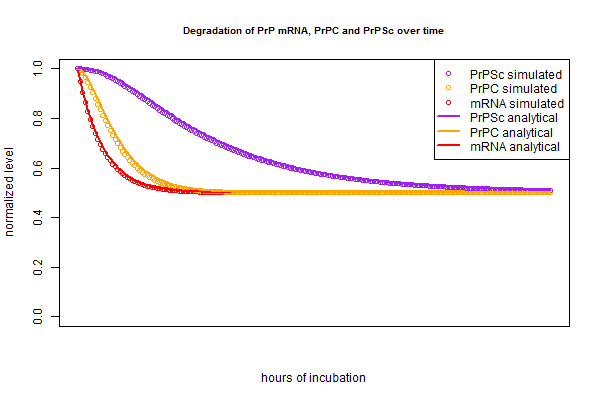
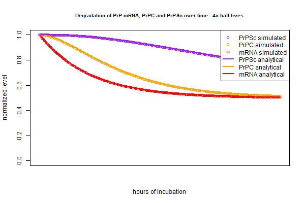
The very slight difference between the circles (simulation) and lines (analytical) is, I believe, analogous to the difference between “period compounding” (simulation) and “continuous compounding” (analytical). If that’s true, then making the compounding periods very fine-grained in the simulation should make the lines closer together. Rather than re-write the whole script to re-define the intervals as 15 minutes instead of 1 hour each, I just tried plugging in new half lives that are 4 times longer, since this is equivalent. And indeed, the simulation and analytical solution are even tighter in this plot:
In the above plots I’ve only considered tweaking one variable – for instance, reducing r with a compound that inhibits PrP mRNA transcription. In chemical screens in real life we’ll only test one compound at a time, but if my models (both simulated and analytical) are correct, they should also be able to predict the kinetics of treating cells with a drug cocktail that, say reduces transcription by half, reduces translation by 30% and doubles the PrPSc degradation rate. Just to check that I’ve got my equations right, let’s try out that scenario:
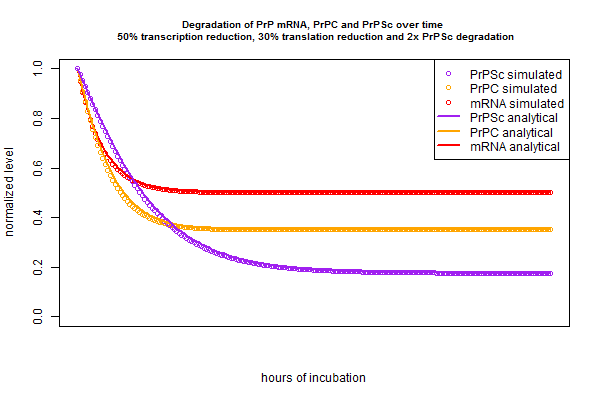
Once again, the simulation and analytical solution agree perfectly. And notice that mRNA’s new steady state is 50% of its original level, PrPC‘s is .5*.7 = 35% of its original level, and PrPSc‘s is .5 * .7 / 2 = 17.5% of its original level.
interpretation
Now, my original purpose in doing the simulation and now in solving these equations was to determine how long you need to incubate cells with candidate antiprion compounds in order to be able to detect compounds with a particular mechanism of action. In published high-throughput screening efforts, people have checked PrPC after 1 day, PrPSc after 5 days or PrPSc after 6 days. Is that enough? I explored this question with plots in my earlier post, but now we can ask the question a bit more rigorously.
We can plug in t1 = 1*24, 5*24 or 6*24 into the equations for R(t), S(t) and T(t) and compare the values of those functions at t1 versus at t = ∞.
We see that, for instance, for compounds inhibiting PrP transcription, only 76% of maximal inhibition in PrPC is achieved by 24 hours.
Though it’s a bit difficult to see from examining the equations for R(t), S(t) and T(t), by playing with the above piece of code I also figured out that these half maximal inhibition values for reducing r, α or β are independent of how much you knock down r, α or β. So if you reduce r by 50%, then you get a 50% reduction in mRNA at t = ∞ and a 50%*76% = 38% reduction at t = 24 hours, just as if you reduce r by 100% (completely shutting off transcription) you get a 100% reduction at t = ∞ and a 76% reduction by t = 24 hours.
For λ, μ and ν, it’s not so simple. If you double λ you will eventually get to a steady state with 50% the original amount of mRNA, and by 24 hours you’ll be at 90% of maximal inhibition. If you multiply λ by 10, then not only will you reach a lower steady state (10% of you original mRNA level), you’ll also get there faster, with 96% of maximal inhibition by t = 24 hours.
discussion
In this post I set out to derive equations to match the simulation I had obtained earlier, and it looks like I’ve achieved that. This still leaves plenty of room open for debate as to whether I have chosen the right model to begin with. The controversial points will be that I haven’t modeled cell division, and I have considered the rate of PrPSc formation to be independent of the amount of PrPSc. I’ll plan to discuss these issues more in a future post.

About Eric Vallabh Minikel
Eric Vallabh Minikel is on a lifelong quest to prevent prion disease. He is a scientist based at the Broad Institute of MIT and Harvard.