A comparison of tools for calling CNVs from sequence data
I’m still getting oriented in my new job at Daniel MacArthur’s lab, and I’m learning that one of the lab’s priorities over the next couple of months will be to improve the way we handle copy number variations (CNVs) in our pipeline for identifying mutations that cause rare Mendelian diseases. We have whole exome (or, in a few cases, whole genome) next generation sequencing (NGS) data for patients and we are exploring using some combination of three different tools for calling CNVs from these NGS data. The three tools in question are ExomeDepth [Plagnol 2012] and XHMM [Fromer 2012] for exomes and GenomeSTRiP [Handsaker 2011] for whole genomes. (Note: there are certainly other tools out there as well – see this Biostars discussion – but these are the ones we’re focusing on here).
In this post I plan to familiarize myself with the three tools in a few different ways:
- the big picture concepts of how they call CNVs and their relative strengths and weaknesses
- how to run them
- how their output is structured
- how they convey confidence and uncertainty in output
The paper introducing ExomeDepth [Plagnol 2012] begins with a nice introduction to CNV calling generally, and defines three distinct approaches to detecting CNVs (or, more broadly, any structural variations) in NGS data:
- split reads – Look for individual reads that span a deletion or insertion breakpoint
- read pairs – Look for read pairs that map to an improbable distance apart (for deletions) or even to different contigs (for structural variations)
- read depth – Look for regions that have too much or too little read depth compared to a reference sample.
Plagnol quickly makes the argument that approaches 1 and 2 are of limited utility in exome sequencing since they’ll only detect breakpoints that happen to fall right within an exon. ExomeDepth is, therefore, based on approach 3.
Read depth depends on many factors besides copy number – alignability, GC content, exome capture efficiency, etc. See my adventures with the PRNP deletions in 1000 Genomes for an example of a false positive CNV call due to GC content. To minimize mistakes like those, read depth should be considered not in absolute terms but relative to a reference sample (say, an average of many other exomes). Other tools were already doing this before ExomeDepth came along, but Plagnol’s main objection to those tools was their assumption that relative read depth should be normally distributed around expectation. Plagnol presents data to refute this assumption and argues for a more complex model based on a beta-binomial model.
ExomeDepth has another clever trick as well, in how it creates a reference sample. Many of the factors I mentioned above – say, GC bias and capture efficiency bias – vary from library prep to library prep, meaning that the best reference sample to compare your test sample to is one which was prepared in the exact same way. That’s hard to achieve. ExomeDepth tries to get as close to this goal as possible by iterating over the samples and progressively selecting as references those individual samples which have the highest correlation (in depth across all exons) with the test sample. So if you’re interested in sample 1, then maybe ExomeDepth will make a reference by averaging sample 9 (r = .99 with sample 1), sample 15 (r = .98), sample 19 (r = .96) and so on, while leaving out sample 2 (r = .87), sample 3 (r = .92), etc. The more samples you add, the lower the variance (since you’re averaging away any real CNVs as well as chance variation in the reference set), but the higher the bias (since you’re adding samples which are less correlated with the test sample). The optimal tradeoff between these countervailing factors seems to occur when using the average of the top 10 or so most correlated samples as a reference.
Even still, ExomeDepth’s power depends massively on just how good the best correlated reference samples are. If there’s a lot of technical variability and only poorly correlated reference samples are available, then no amount of read depth will give you adequate power. This point was argued again in a blog post from the Plagnol lab.
In terms of strengths and weaknesses, ExomeDepth is really at its shining best when you have a number of highly correlated samples – i.e. samples prepared in almost exactly the same way. As pointed out in the vignette, those samples also need to not have the CNV you’re interested in, which means that you need unrelated samples and you’re best off if you’re looking for rare CNVs (e.g. in Mendelian disorders) rather than common CNVs.
ExomeDepth is implemented as an R package with a handy vignette. For input, you need BAMs aligned to hg19, sorted and index. ExomeDepth will take it from there – calculating depth for each exon, selecting a reference set and calling CNVs. I’ve got a simple R script to run ExomeDepth up and running here. By way of exposition, the two basic steps are as follows. First, pass a vector of BAM path strings to getBamCounts to get counts per sample per exon:
counts = getBamCounts(bed.frame = exons.hg19, bam.files = bams)
Here’s an easy thing to get tripped up on: when you first read that list of BAMs in from disk, it is *essential* that you have set options(stringsAsFactors=FALSE) so that the getBamCounts function sees strings, not factors.
Next, iterate over the samples you want to call CNVs on, and for each one, find the best reference set and then call CNVs against those. Note that (as far as I can tell) you end up needing three copies of the counts: one as its native S4 object, one as a data frame and one as a matrix. Let me know if you have a way to avoid this.
countdf = as.data.frame(counts)
countmat = as.matrix(countdf[,6:dim(countdf)[2]]) # remove cols 1-5 metadata

for (i in 1:dim(countmat)[2]) {
    sample_name = colnames(countmat)[i]
    reference_list = select.reference.set(test.counts = countmat[,i],
        reference.count = countmat[,-i],
        bin.length=(countdf$end-countdf$start)/1000,
        n.bins.reduced = 10000)
    reference_set = apply(
        X = as.matrix(countdf[, reference_list$reference.choice]),
        MAR=1, FUN=sum)
    all_exons = new('ExomeDepth', test=countmat[,i],
        reference=reference_set,
        formula = 'cbind(test,reference) ~ 1')
    all_exons = CallCNVs(x = all_exons, transition.probability=10^-4,
        chromosome=countdf$space, start=countdf$start,
        end=countdf$end, name=countdf$names)
    write.table(all_exons@CNV.calls, file=paste(sample_name,".txt",sep=''),
        sep='\t', row.names=FALSE, col.names=TRUE, quote=FALSE)
    if (opt$verbose) {
        cat(paste("Wrote CNV calls for ",sample_name,"\n",sep=''),file=stdout())
    }
}
The output for each sample will look like this (formatted with cat samplename.bam.txt | column -t):
start.p  end.p   type         nexons  start     end       chromosome  id                       BF    reads.expected  reads.observed  reads.ratio
231958   231958  deletion     1       16287256  16287718  22          chr22:16287256-16287718  38.1  223             0               0
232036   232037  deletion     2       17061818  17062178  22          chr22:17061818-17062178  5.55  205             123             0.6
232070   232070  duplication  1       17177670  17179047  22          chr22:17177670-17179047  5.71  61              124             2.03
The CNVs are identified by genomic coordinates. There’s also an option to annotate them with IDs from Conrad 2010 (a paper with some validated CNVs) and exon IDs, but this is in beta.
The output includes a BF column, for Bayes Factor. In theory this the log10 likelihood ratio of the alternative hypothesis (yes there’s a CNV) over the null hypothesis (no CNV here) — so in the first row above, the CNV is 1038 more likely than no CNV — though the vignette acknowledges these may sometimes be “unconvincing”. ExomeDepth describes itself as being “aggressive” [see vignette] – i.e. it favors sensitivity in its CNV calls, and if you want specificity instead, the Bayes Factor is there for you.
In terms of runtime, for a toy example to get started with I subsetted out only chromosome 22 from 20 BAMs, computed counts and called CNVs on all of them. This tiny task took 38 minutes in total. Note that I did the CNV calling in serial, whereas you could easily save off the counts to an .rda file and then parallelize the CNV calling part.
Like ExomeDepth, XHMM [Fromer 2012, see also this presentation] relies on read depth as the sole source of information on CNV events, ignoring split read and read pair information. But whereas ExomeDepth creates an optimized reference sample set to handle all the sources of inter-exon variability, XHMM uses principal components to handle normalization. In particular, it creates a matrix of the depth of all exons in all samples, and the principal components of this matrix are expected to capture many of the non-CNV factors that affect an exon’s read depth.
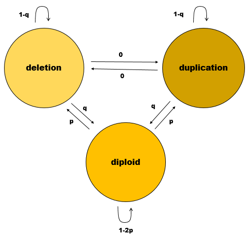
Once normalization is done and XHMM gets around to calling CNVs, it does something clever, as you may have guessed from the name, which stands for exome hidden Markov model. Whereas ExomeDepth considers every exon as being completely independent of every other exon, XHMM takes advantage of the fact that (sufficiently large) CNVs will affect a whole contiguous swath of exons. In other words, if exon 1 is deleted, then the prior probability for exon 2 being deleted is considerably higher than if no CNV had yet been detected in the gene. Hidden Markov models rely on probabilities of transitions between states (e.g. from the “no CNV” state to the “yes CNV” state and back again), and the XHMM needs just two quantities from which to base all of its probabilities. p is the rate of exonic CNVs, and q is the reciprocal of the average CNV length (number of exons). According to Table 1, the model assumed is this:
Like ExomeDepth, XHMM is tuned to detect rare CNVs, whereas common CNVs may go undetected since they are present in the reference samples used for PCA. Also like ExomeDepth, XHMM favors sensitivity over specificity in its calling process, giving you a long list of possible CNVs along with quality scores so that you can filter as you wish. The quality scores are the posterior probabilities for each CNV as per HMM theory.
XHMM was developed by the folks at Broad, and accordingly it is built around GATK – the user is expected to first run GATK’s DepthOfCoverage function to get exon read depths. Like GATK, XHMM is non-trivial to use. The authors have provided a 70-minute YouTube tutorial:
My most basic pipeline to run XHMM right now is this bash script. My goal with it was just to see what it would take to get XHMM to run at all; there’s nothing good or interesting about the way I’m running it and I’m not using any of the fancy options. It’s basically a very lightly modified version of some getopts code to accept command line args from this StackOverflow post and the example code from the XHMM tutorial. One trivial but useful point: your BAM list must have a name that ends in .list.
As you can see from that bash script, it takes a lot more code to run XHMM than to run ExomeDepth. Once you do, the outputs are two. You get a VCF file with the CNV boundaries as the ID field, <DIP> (for diploid) as the REF field, and <DEL>,<DUP> (for deleted/duplicated) as the ALT field, like so:
#CHROM  POS       ID                    REF    ALT          QUAL  FILTER  INFO
22      23029456  22:23029456-23241835  <DIP>  <DEL>,<DUP>  .     .       AC=1,0...
22      23077281  22:23077281-23165783  <DIP>  <DEL>,<DUP>  .     .       AC=3,1...
22      23077281  22:23077281-23223572  <DIP>  <DEL>,<DUP>  .     .       AC=3,0...
And you also get a .xcnv file where each row is one sample-CNV combination, with all manner of quality scores included as columns for your filtering pleasure:
SAMPLE      CNV  INTERVAL              KB      CHR  MID_BP    TARGETS     NUM_TARG  Q_EXACT  Q_SOME  Q_NON_DIPLOID  Q_START  Q_STOP  MEAN_RD  MEAN_ORIG_RD
sample1     DEL  22:23077281-23247205  169.93  22   23162243  579..594    16        25       99      99             33       12      -3.52    38.07
sample2     DEL  22:39378457-39388452  10.00   22   39383454  2097..2104  8         3        99      99             3        3       -3.88    30.50
sample3     DEL  22:23029456-23241835  212.38  22   23135645  574..592    19        10       99      99             16       9       -3.77    28.84
sample4     DUP  22:23077281-23165783  88.50   22   23121532  579..587    9         21       71      71             23       17      2.90     89.04
The (sadly paywalled) GenomeSTRiP paper [Handsaker 2011] provides an almost narrative walk-through of the logic that went into designing it. Unlike the exome-based callers above, GenomeSTRiP utilizes all three possible sources of CNV information: read pairs, split reads, and read depth.
The paper goes into the greatest detail on how aberrant read pairs – those which map too far apart, suggesting a deletion in between them – are utilized. To maximize statistical power, it uses three concepts which the authors introduce as coherence, heterogeneity, and allelic substitution.
- coherence means that the statistical case for a CNV is based on cumulative evidence from many read pairs in many genomes. While chimeric molecules generated in the sequencing process should be dispersed across the genome, read pairs representing true CNV breakpoints should be clustered in one place. Moreover, in high-n-but-low-coverage sequencing projects like 1000 Genomes, aberrant read pairs for not-too-rare CNVs should be found in many different genomes, so you get more power from populaton-based (rather than individual) CNV calling. (However, it is noted that GenomeSTRiP still can call CNVs private to one individual).
- heterogeneity means that if the CNV is real, then some genomes have it and others don’t, and those cases should look different. 1 aberrant read pair in each of 50 genomes looks like noise; 50 aberrant read pairs in 1 genome looks real. GenomeSTRiP applies a chi squared test of independence to determine whether aberrant read pairs at a particular site occur equally in all genomes or are clustered in a few genomes.
- allelic substitution means that if Haplotype A contains a deletion and Haplotype B doesn’t, then across genomes, the abundance of reads supporting Hap A should be inversely correlated with the abundance of reads supporting Hap B.
This tutorial helped me to understand that GenomeSTRiP actually operates in a few distinct phases: discovery, refinement and genotyping.
- discovery. The above-described tricks, based on read pairs, are all used to discover CNVs in a population of samples. As a validation of sorts, the average read depth over the putative CNV site is then compared between samples with aberrant read pairs and those without. Proposed CNVs are written to a library file.
- refinement. The proposed CNVs from the genotyping stage are validated by de novo assembly of nearby (and/or unmapped) reads to see if any turn out to be split reads spanning a breakpoint. Unfortunately, GenomeSTRiP doesn’t quite do this all for you. They recommend using a third-party tool (TIGRA-SV [Chen 2014] or AGE [Abyzov & Gerstein 2011]) to discover the exact alternate alleles and get a VCF, and then GenomeSTRiP will use that VCF and your BAMs to re-align reads from your samples to the proposed alternate alleles.
- genotyping. Each sample is tested for evidence – from read pairs, split reads and read depth – of the validated CNV haplotypes from the refinement stage.
Reading through the tutorial, it strikes me that many of the parameters used by GenomeSTRiP under default settings are chosen for low-depth, high-n studies like 1000 Genomes. For instance, the default threshold for discovery is a minimum of 1.1 aberrant read pairs per proposed affected samples [tutorial]. If you’ve got decent depth, you can afford to set a much higher threshold than that, and if you’ve got low n, you need to.
Towards the end of the tutorial there is more discussion of how to apply GenomeSTRiP to Mendelian families with low n. In general, GenomeSTRiP is said to “Need 20-30+ samples for good results”, and calling variants in a single deeply sequenced individual is still a “Future goal.” But if you do manage to call some variants in a small family with a rare Mendelian disease, one nice facility that GenomeSTRiP provides is the ability to check for the presence of your variant in the 1000 Genomes BAM, to confirm its rareness.
GenomeSTRiP is by far the most complex of the three tools described here, and accordingly its operation has so far eluded me altogether. The official documentation provides four separate Queue scripts for running the various steps of GenomeSTRiP; the cookbook only has examples of the (comparatively) simple task of genotyping a known site in 1000 Genomes. My past experience with Queue tells me it would probably take me tens of hours to get competent at using GenomeSTRiP – this is the kind of investment that shouldn’t be duplicated, so I’m going to hold off for bigger plan on how we’ll run GenomeSTRiP before diving into it myself.
how to use all three tools?
Say we have – best case scenario – both exome and whole genome data on some samples, and we want to run all three tools. They are each looking at sources of information that are at least partly orthogonal, so they each could bring valuable information to the search for a causal CNV in a patient. Our current thinking is not to try to do any meta-analysis of the three outputs, but rather to just list (say, for each exon) whether each tool called a CNV, and with what quality/probabilty, etc.

About Eric Vallabh Minikel
Eric Vallabh Minikel is on a lifelong quest to prevent prion disease. He is a scientist based at the Broad Institute of MIT and Harvard.