Genetics 03: 'Linkage and tetrad analysis in yeast'
These are my notes from lecture 03 of Harvard’s Genetics 201 course, delivered by Fred Winston on September 8, 2014.
Here are some key review points from last time:
- We discussed 2 methods for isolating haploid CisR mutants.
- Tests of dominance vs. recessiveness must be done in diploids.
- Complementation is done only in recessive phenotypes and tests the function of two mutations.
Simple complementation example
Suppose we isolate two mutants, trp1 and trp2 in the tryptophan biosynthetic pathway. Each of them causes the haploid cell to be unable to produce tryptophan, a phenotype designated Trp-. We see the following genotype-phenotype relationships in diploids.
| diploid genotype | phenotype | conclusions |
|---|---|---|
| TRP1/trp1 | Trp+ | trp1 is recessive |
| TRP2/trp2 | Trp+ | trp2 is recessive |
| trp1/trp1 TRP2/TRP2 | Trp- | no complementation |
| TRP1/trp1 trp2/TRP2 | Trp+ | complementation |
The first two rows are crosses to wild-type which are called “dominance/recessiveness tests”. In this case, the dominance/recessiveness tests show that both mutants are recessive. The last two rows are crosses of mutants which are called “complementation tests”. In this case, the results of the complementation test demonstrate that TRP1 and TRP2 are separate complementation groups, and therefore probably (with below-listed exceptions) separate genes.
But sometimes reality is more complex.
Sometimes complementation can give misleading results [Hawley 2006]. Here are two examples.
Intragenic complementation
Mutant hunts and complementation screens for histidine biosynthesis revealed three complementation groups: his4A, his4B and his4C. These all complemented each other, but were shown to be in extremely tight genetic linkage. It eventually turned out that the yeast protein HIS4 is one protein with three activities mediated by three separate domains, and that the three mutations fell in the three domains responsible for the 3rd, 2nd and 10th steps of histidine biosynthesis respectively. Today, this could have been discovered by sequencing the causal mutations, but this occurred in the pre-genomic era, so the researchers actually had to do biochemistry and show that the enzymatic activities of all three complementation groups co-purified with the same protein. This phenomenon is called intragenic complementation.
Unlinked noncomplementation
Sometimes two recessive mutations in different genes fail to complement each other. This reveals itself to the researcher as follows: the genes can be shown to be unlinked, but the complementation results are as follows:
| diploid genotype | phenotype |
|---|---|
| +/+ | wt |
| +/cis1 | wt |
| +/cis5 | wt |
| +/cis1, +/cis5 | mutant |
There can be a few explanations. One possible mechanism is that the two proteins act as a complex, and the level of the complex is proportional to the levels of all constituent proteins. So if you knock down two components by 50% you only get 25% of the complex’s function, and let’s say the threshold of complex activity required for a wild-type phenotype is 30%.
This phenomenon, called unlinked noncomplementation, has also been observed in human disease - a famous example is retinitis pigmentosa [Kajiwara 1994].
Linkage
Thomas Hunt Morgan noticed that there were more independently segregating groups of traits than there were chromosomes. A proposed explanation was that genes could be exchanged between sister chromatids during meiosis - “crossovers” or “recombination”. He hypothesized that the degree of linkage corresponded to the physical distance of genes along a chromosome.
In yeast, linkage is studied through tetrad analysis.
Tetrad analysis
Tetrad analysis is used in yeast for:
- Mutant analysis
- Location of mutations
- Cloning a gene
- Strain construction
- Whole-genome sequencing
Suppose we follow a cis1 mutation through meiosis. We begin with an a CIS1 haploid cell and an α cis1 haploid cell. We obtain CIS1/cis1 diploids, which can then go through sporulation (meiosis) which includes DNA replication in the premeiotic S phase. Following the replication, the cell has four “strands” - four chromatids, or four homologous copies, each of double-stranded DNA. This is called the “4-strand stage”. This is metaphase, but it is special - metaphase during yeast meiosis involves all four homologous copies of each chromosome lining up together, whereas during mitosis, only two sisters need to align. Recombination occurs at this stage of meiosis (between non-sister chromatids, otherwise it wouldn’t generate any diversity), and pairs connected at a centromere are called sister chromatids. Then Meiosis I occurs, and sisters segregate together. In Meiosis II, sisters segregate apart, yielding four haploid products.

The four offspring are then dissected to perform tetrad analysis. One expects a 2:2 Mendelian segregation of alleles. This allows you to determine the number of mutations responsible for a phenotype, and to test the position of genes relative to each other and to the centromere.
To determine if a trait is Mendelian, do a cross and look for a 2:2 ratio. If you cross cis9 × wt and get 2:2 of each phenotype, then the phenotype is likely caused by a single mutation; if not, then it’s probably a more complex, non-Mendelian trait.
The process for determining whether a trait is monogenic and Mendelian is nearly the same in peas, or mice, or any other model organism. Obtain pure-bred lines, cross with wild-type, self the F1s, and if you obtain a 3:1 ratio in the F2s, then you have a Mendelian trait.
Now consider a cross of unlinked markers A and B. Cross a AB × α ab. In the absence of recombination, you will get two types of tetrads: AB AB ab ab tetrads and Ab Ab aB aB tetrads. The former is called parental ditype (PD) and the latter is called non-parental ditype (NPD). If A and B are unlinked, PD and NPD will occur in a 1:1 ratio. (In reality, recombination does occur, so the unlinked markers will also have recombinants (“tetratype”, see below, and their frequency is related to the distance of A and B from the centromere), but after removing these, the remaining offspring will be PD:NPD in a 1:1 ratio. Whereas if A and B are linked, PD > NPD.
If we additionally consider recombination, we could get a third outcome, neither PD nor NPD, called tetratype (TT): an AB Ab aB ab tetrad. The three outcomes are sometimes abbreviated P, N, and T. Suppose we cross AB × ab and analyze 100 tetrads, and get 90 PD, 0 NPD, and 10 TT. Linkage is measured as the number of recombinants divided by the total progeny. Because there are four progeny per tetrad, here we have 400 spores, and 2 of the 4 in each TT tetrad are recombinants. Therefore we have 20 recombinants out of 400 = 5% recombination or 5% linkage. This is called 5 centiMorgans (cM). 1 cM is defined as 1% recombination.
In terms of tetrads, ½T/(T+N+P) × 100 = number of cM. Yeast, however, have so much recombination that you often see double crossovers (DCOs). There are only four unique types:
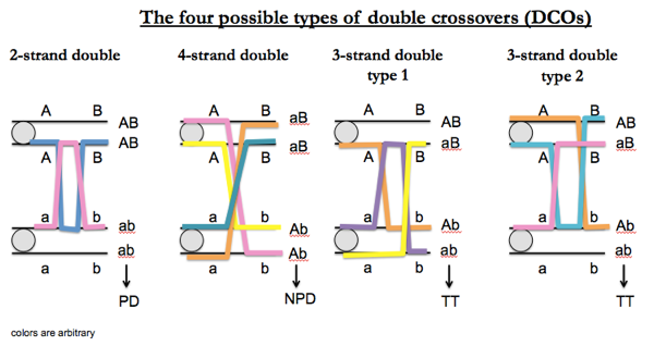
For linked markers, NPD outcomes can only be obtained in DCOs. In fact, for all possible DCOs (the four equally likely outcomes diagrammed above), P:N:T = 1:1:2. For linked markers, types of tetrads can be produced by different numbers of crossover events as follows:
| tetrad | number of crossovers |
|---|---|
| PD | 0 or 2 |
| NPD | 2 only |
| TT | 1 or 2 |
For clarity, it is worth repeating that the above table applies only to linked markers. For unlinked markers, all three outcomes (PD, NPD and TT) are possible.
Getting back to linked markers, remember that single crossovers give rise to 100% T outcomes. DCOs, as stated above, give rise to P:N:T in a 1:1:2 ratio. Therefore it is a rule that NPDs are 1/4 of the total number of DCOs for linked markers. Because NPDs arise only as a result of double crossover for linked genes, it is useful to express the formula in terms of NPDs. Therefore we can state the following quantities:
- Number of tetrads with a DCO = 4N
- Number of tetrads with a SCO = T - 2N
- Total number of recombinants = 2(4N) + (T-2N) = 6N + T
The number of tetrads with a SCO is T - 2N because there are a total of T tetratypes, but 2N of those are from DCOs, while the rest must be from SCOs, which give rise exclusively to T. Note that Fred calls the last quantity (6N +T) the “total number of recombiants,” which I found slightly confusing. I asked Fred after class and he explained that this can be thought of as the number of recombination events (where a single counts as 1 and a double counts as 2), and if you multiply it by 4, you get the number of spores that harbor a recombinant chromosome.
The recombination frequency in centiMorgans, then, is 100 × ½(6N+T)/(P+N+T).
This formula is valid for distances up to about 35 cM.
In yeast, 1 cM is about 2.5 kb.
After you do a cross, first check whether PD == NPD. If yes, then the markers are unlinked, and you don’t need to do anything else. If PD > NPD, then the markers are linked, and you can compute a recombination frequency as 100 × ½(6N+T)/(P+N+T). If PD < NPD, you’re probably #DoingItWrong.

About Eric Vallabh Minikel
Eric Vallabh Minikel is on a lifelong quest to prevent prion disease. He is a scientist based at the Broad Institute of MIT and Harvard.