Some musings on age of death in FamiLinx
Last fall at the American Society of Human Genetics meeting in Boston, I got to see Yaniv Erlich introduce FamiLinx, a most remarkable dataset. Compiled from data entered by the recreational genealogy enthusiasts who use Geni.com, FamiLinx contains basic biographical details — year of birth, death, location, family structure — for >43 million people. He has made the de-identified data free to download prior to publication.
Shortly after hearing him speak, I downloaded the dataset to have a look myself. At the time, I was working on a study of how ascertainment bias affects analyses of age of onset (or death) in genetic disease, and I suspected that some of the same biases we saw in our data would also apply to age of death of any cause. Sure enough, I found some interesting parallels between FamiLinx and the dataset I was working on. My own study was published last week [Minikel 2014], but I did not include any of the analyses of Yaniv Erlich’s data because FamiLinx is still under Ft. Lauderdale embargo until publication. But that doesn’t prohibit blogging about FamiLinx (and to be sure, I also asked Yaniv Erlich for his permission) so in this post I’ll present a few of the interesting things I observed in FamiLinx.
For background, it’s good to define a couple of terms up front:
- Anticipation is the phenomenon where a genetic disease strikes younger or more severely in successive generations.
- Heritability is the proportion of a phenotype’s variation that can be explained by genetic factors. This post reviews some methods for estimating heritabilty.
In my new paper [Minikel 2014] we showed that the “anticipation” reported in E200K genetic prion disease was an artifact due to ascertainment bias. See my last post for a simple overview of the logic. An essential point was that the vast majority of our data points for E200K genetic prion disease were from individuals who died between 1989 (the year the mutation was discovered) and 2013 (the last year we collected data). You can’t get age of death for people who live healthily past 2013 because they’re still alive. And it is difficult to get age of death for people who died before 1989 because hardly anyone was collecting data on these families at the time. You can fill in some of that old data retrospectively, but family histories aren’t always collected, and even when they are, they are not always perfect - details get lost, diagnoses are uncertain.
In our study we performed paired t tests on age of onset (or death) in parent-child pairs with the E200K mutation (not the correct statistical test to use here, but we were mirroring the methods of the studies we were refuting). Nominally, we did see “anticipation”: children died of the disease 7 to 28 years younger than their parents. But we were able to show that this was an artifact. An important negative control was that even among unaffected individuals in these families, children died — of any cause — 14 to 35 years younger than their parents did. We argued that if even unaffected individuals show “anticipation”, then the anticipation is surely related to ascertainment bias and not a biological feature of the disease caused by the E200K mutation.
With that in mind, the first thing I set out to check in FamiLinx was whether children died younger than their parents. I exported from MySQL the data on all of the parent-child pairs where year of birth and death were available for both parent and child.
-- query to generate all parent-child pairs
select   r.Child_id child_id, r.Parent_id parent_id,
         (yc.Dyear - yc.Byear) child_ad, (yp.Dyear - yp.Byear) parent_ad, -- ages of death
         yc.Byear child_yob, yp.Byear parent_yob, -- years of birth
         yc.Dyear child_yod, yp.Dyear parent_yod -- years of death
from     relationship r, years yc, years yp
where    r.Child_id = yc.Id
and      r.Parent_id = yp.Id
and      yc.Byear > -1 and yc.Dyear > -1 -- can't compute age of death if either birth year or death year is unknown (-1)
and      yp.Byear > -1 and yp.Dyear > -1
into outfile '/humgen/atgu1/fs03/eminikel/039famil/parent-child-pairs.txt'
;
Switching to R, I performed some basic QC:
# parent-child ("pc") pairs
pc = read.table('/humgen/atgu1/fs03/eminikel/039famil/parent-child-pairs.txt',header=FALSE,sep='\t')
colnames(pc) = c('child_id','parent_id','child_ad','parent_ad','child_yob','parent_yob','child_yod','parent_yod')

# basic sanity check on parent/child ages of death - should all be between 0 and 120,
# and parent should not die before child is born (-1 to allow rare cases of father dying after conception)
error_free_pairs = pc$child_ad >= 0 & pc$child_ad <= 120 & pc$parent_ad >=0 & pc$parent_ad <= 120 & pc$parent_yod >= pc$child_yob - 1
sum(!error_free_pairs) # check the number of pairs that appear to have errors
pc = pc[error_free_pairs,] # remove the errors
And then a paired t test on age of death in all parent-child pairs. Sure enough, there were 14 years of “anticipation” between parent and child:
    Paired t-test

data:  pc$parent_ad and pc$child_ad
t = 533.6126, df = 1435459, p-value < 2.2e-16
alternative hypothesis: true difference in means is not equal to 0
95 percent confidence interval:
 13.80287 13.90464
sample estimates:
mean of the differences
               13.85376
At first glance this seems pretty non-intuitive: life expectancy has been on the rise for most of recent human history, so surely children should be living longer than their parents. But as pointed out in the seminal work on anticipation [Penrose 1948], everyone is someone’s child, but people who die young never become someone’s parent. The fact that the world contains parent-child pairs where the child dies in infancy, but no pairs where the parent dies in infancy, means that a paired t test will inevitably uncover a younger age of death for children than their parents. Was this the source of “anticipation” in FamiLinx? I sought to answer this question by setting different minimum age thresholds for including parents and children in the paired t test. For instance, consider a minimum age of 40: if we include only pairs where both parent and child survived to at least age 40, then we’ve ensured that the child at least had an opportunity to reproduce and didn’t die in infancy. I therefore computed the paired difference in age of death for FamiLinx parent-child pairs with every possible minimum age threshold from 0 to 80 to see how this would affect “anticipation”:
anticipation_vs_min_age = data.frame(min_age_of_death=integer(0),anticipation=numeric(0),p=numeric(0))
for (min_age_of_death in 0:80) { # for every possible minimum age threshold, 0 to 80
    subset = pc$child_ad >= min_age_of_death & pc$parent_ad >= min_age_of_death # only include pairs where both survived to minimum age
    t_test_result = t.test(pc$parent_ad[subset], pc$child_ad[subset], paired=TRUE, alternative='two.sided')
    anticipation = as.numeric(t_test_result$estimate) # mean paired difference
    p = as.numeric(t_test_result$p.value) # p value for there being a difference
    anticipation_vs_min_age = rbind(anticipation_vs_min_age, c(min_age_of_death,anticipation,p))
}
Here are the results:
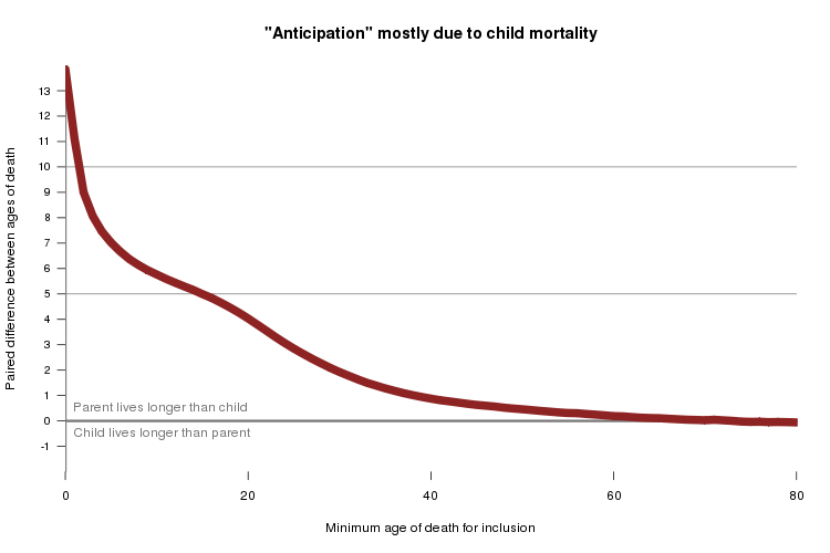
As I suspected, most of the difference in parent and child was due to child mortality. The 14 year difference among all individuals drops to about 5 years if you consider only pairs where both parent and child survived to at least age 15. If you only consider pairs where both parent and child had ample opportunity to reproduce, living to at least age 40, the difference drops to only about 1 year.
Yet that 1 year difference is still highly significant (p < 1e-15). With millions of data points, practically everything is signficant, the question is whether it means anything real. I hypothesize that this 1 year difference reflects recall bias: although parents who die young will of course be remembered by their own children, they are somewhat less likely to be remembered in detail by their grandchildren or great-grandchildren who grow up to be Geni.com users. In the negative controls in our E200K study, we found that even when we considered only unaffected parent-child pairs where both individuals survived to at least 40, we still saw 16 years of “anticipation”. I suspect that’s because people of my generation - often the ones giving family history to the clinicians who collect these data - will remember a relative who died young in 2000 but will be fuzzy on details about a relative who died young before we were born. Thus you can more readily collect family history data on parent-child pairs where the child died young (which would have happened recently) than on pairs where the parent died young (which happened a long time ago). My own knowledge of my family’s genealogy is embarrassingly bad, and the 16-year of “anticipation” in the unaffected members of E200K famiilies probably reflects similarly poor recall. Recreational genealogy enthusiasts know a heck of a lot more about their family history, and that’s why the FamiLinx data are so good that you only see 1 year of anticipation in the survived-to-at-least-40 analysis. That’s my hypothesis - but there are probably several other sources of bias which could help to explain the “anticipation” in FamiLinx, and I haven’t explored it in detail.
It’s tough to talk about anticipation, though, without also talking explicitly about year of birth. I went back to MySQL and exported the year of birth and year of death data for everyone who had them:
-- query to just get year of birth, year of death and age of death for everyone possible
select   y.Byear yob, -- year of birth
         y.Dyear yod, -- year of death
         (y.Dyear - y.Byear) ad -- age of death
from     years y
where    y.Byear > -1
and      y.Dyear > -1
into outfile '/humgen/atgu1/fs03/eminikel/039famil/yob-yod-ad.txt'
;
Consider this plot of age of death versus year of death:
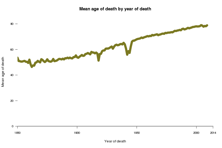
This is probably what you expected for a plot of longevity over time: a nearly monotonic rise in life expectancy, with a couple of dips corresponding to world wars. Yaniv Erlich showed a plot similar to this at ASHG2013, and this is also similar to how life expectancy is calculated. For instance, the Social Security 2010 Life Tables are based on the mortality statistics of all of the people who died in 2010, regardless of when they were born.
Now, if you instead plot age of death versus year of birth, you see a very different picture:
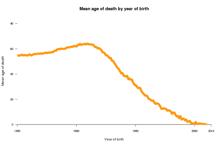
You can see age of death rising gradually between 1850 and about 1910 (probably reflecting increases in life expectancy), and then it starts to decline precipitously - by the year 2000, the average age of death is less than 1 year. That’s because people born in 2000 had to die young, or else they wouldn’t have an age of death in this dataset yet. As a result of this unavoidable source of ascertainment bias, even apart from any changes in life expectancy, year of birth and age of death will be artifactually correlated in any real dataset.
It’s also true that a parent’s year of birth is correlated with their child’s year of birth - people born in the 1920s had kids in the 1950s, people born in the 1950s had kids in the 1980s, and so on. In FamiLinx, the Pearson’s correlation between parent and child year of birth is rho = .99.
    Pearson's product-moment correlation

data:  pc$child_yob and pc$parent_yob
t = 10804.88, df = 1435458, p-value < 2.2e-16
alternative hypothesis: true correlation is not equal to 0
95 percent confidence interval:
 0.9938884 0.9939281
sample estimates:
      cor
0.9939083
Now, consider this. Year of birth and age of death are correlated (as the above plot shows). Parent and child year of birth are also correlated (as this Pearson’s correlation shows). As a result, parent and child age of death can become correlated simply as a result of ascertainment bias. That observation is nothing new [see Penrose 1948], but FamiLinx is a useful reminder that this is a big problem for estimation of heritability. As defined above, heritability refers to the genetic contribution to a trait. Parent-offspring regression considered to be one method for estimating heritability [Visscher 2008] - for one parent vs. one child, you simply double the slope of the regresion line and that’s your additve heritability (h2). This core concept has been applied, in various incarnations and models, to the task of estimating the heritability of age of onset in a number of genetic diseases - for instance Huntington’s disease [Wexler 2004] and early-onset Alzheimer’s disease [Ryman 2014].
In our recent paper [Minikel 2014] we showed in a simulation that ascertainment bias alone could be enough to lead to an estimate of heritability over 100%, even when a trait is not at all heritable. We suggested that when one performs a regression analysis on parent age of onset (or death) and child age of onset (or death), it may be wise to including a child’s year of birth as a covariate. In other words, instead of just:
m = lm(pc$child_ad ~ pc$parent_ad)
I’d throw in child year of birth as well:
m = lm(pc$child_ad ~ pc$parent_ad + pc$child_yob)
I thought the longevity data in FamiLinx would make an interesting test case for this framework. There is plenty of evidence from well-designed studies showing that longevity really truly is a heritable trait - for instance, a large twin study with virtually complete ascertainment reported ~25% heritability [Herskind 1996]. Yet as shown above, year of birth and age of death in FamiLinx exhibit a surprising correlation which is clearly related to ascertainment and not biology. One could imagine that would inflate heritability estimates. So does a simple estimate of the heritability of longevity based on parent-offspring regression change if we throw in a year of birth covariate?
Here are the results without a year of birth covariate:
Call:
lm(formula = pc$child_ad ~ pc$parent_ad)

Residuals:
    Min      1Q  Median      3Q     Max
-63.977 -19.824   8.352  22.352  77.916

Coefficients:
              Estimate Std. Error t value Pr(>|t|)
(Intercept)  40.083640   0.104504   383.6   <2e-16 ***
pc$parent_ad  0.205974   0.001498   137.5   <2e-16 ***
---
Signif. codes:  0 ‘***’ 0.001 ‘**’ 0.01 ‘*’ 0.05 ‘.’ 0.1 ‘ ’ 1

Residual standard error: 28.45 on 1435458 degrees of freedom
Multiple R-squared:  0.013, Adjusted R-squared:  0.013
F-statistic: 1.89e+04 on 1 and 1435458 DF,  p-value: < 2.2e-16
And with:
Call:
lm(formula = pc$child_ad ~ pc$parent_ad + pc$child_yob)

Residuals:
   Min     1Q Median     3Q    Max
-71.43 -19.98   8.26  22.39  77.88

Coefficients:
               Estimate Std. Error t value Pr(>|t|)
(Intercept)  53.3302896  0.4108069  129.82   <2e-16 ***
pc$parent_ad  0.2138382  0.0015161  141.05   <2e-16 ***
pc$child_yob -0.0075818  0.0002274  -33.34   <2e-16 ***
---
Signif. codes:  0 ‘***’ 0.001 ‘**’ 0.01 ‘*’ 0.05 ‘.’ 0.1 ‘ ’ 1

Residual standard error: 28.44 on 1435457 degrees of freedom
Multiple R-squared:  0.01376,   Adjusted R-squared:  0.01376
F-statistic: 1.001e+04 on 2 and 1435457 DF,  p-value: < 2.2e-16
When we add the year of birth covariate to the model, the coefficient for parent age of death actually rises from .206 to .214 - meaning the estimate of heritability by this crude method rises from 41% to 43%. It is comforting to see that, at least for one trait we know is really heritable, adding this year of birth covariate actually strengthens the correlation between parent and child year of birth.
Of course, this is just one dataset and I can’t say how well that result would translate to the small N, less thoroughly ascertained datasets we typically see in rare genetic diseases. Those sorts of datasets are the only ones where I’ve actually seen anyone use a simple parent-offspring regression to estimate heritability — for larger datasets and especially for datasets with SNP genotyping data, you have more sophisticated tools available such as GCTA [Yang 2011].
And with a dataset as large as FamiLinx, of course, there exists a whole world of questions one can ask about heritability - I haven’t begun to scratch the surface here. Yet even the pretty superficial analysis in this blog post has helped to shape some of my thinking, though, so +1 to Yaniv Erlich for sharing this dataset ahead of publication!
I’ll end with a self-promotion. If this sounds interesting and you’re attending ASHG2014 in San Diego in a couple of weeks, you should come to the crowdsourced genetics session at 10:00a - 12:00p on Sunday, Oct 19 in Room 6AB, Upper Level, Convention Center. Yaniv Erlich will be presenting on FamiLinx (“crowd mining”), and if what I’ve seen so far is any guide, his presentation will include some really sophisticated analyses on the heritabilty of longevity using this dataset. And I and my wife Sonia will be presenting on the crowdfunding project we undertook last year to fund preclinical trials of a drug candidate for genetic prion disease. See you there!
All source code for this post is here.

About Eric Vallabh Minikel
Eric Vallabh Minikel is on a lifelong quest to prevent prion disease. He is a scientist based at the Broad Institute of MIT and Harvard.