New Technologies Club lecture on cryo-electron microscopy
These are my notes from a lecture by Youdong (Jack) Mao from Harvard Medical School, at the Broad’s New Technologies Club Meeting on Friday, June 3, 2016. Note that I don’t understand structural biology all that well, and my notes are likely to contain some errors.
The purpose of today’s lecture is to introduce new advances in cryo-electron microscopy and how you can use them to solve protein structures.
Here are the steps for a cryo-EM experiment:
- Sample preparation and purification. The protein needs to be soluble, and at just the right concentration that you can see single molecules.
- Vitrification — fast cooling (105 °K/s) into very thin vitreous ice
- Data collection by transmission EM
- Image processing
- Data interpretation
Fast cooling allows you to obtain vitreous ice, which is different from crystalline ice. If you freeze at a normal rate, the water molecules form a hexagonal lattice, with one of 16 different patterns (yes, there are different ices in real life, not just in Cat’s Cradle). If you freeze so fast that the water molecules don’t have time to rearrange into a lattice, you get a solid without any long-range ordered structure.
Typical conditions are 2-3μL of a 1-2 mg/mL protein solution, applied to an EM grid and plunged into liquid ethane (-160°C) within 1 millisecond and then kept at liquid nitrogen temperatures for the duration of the experiment. The most common error mode for cryo-EM experiments is to get crystalline ice contamination into your sample at some point int his process.
This process allows you to literally obtain images of single protein molecules.
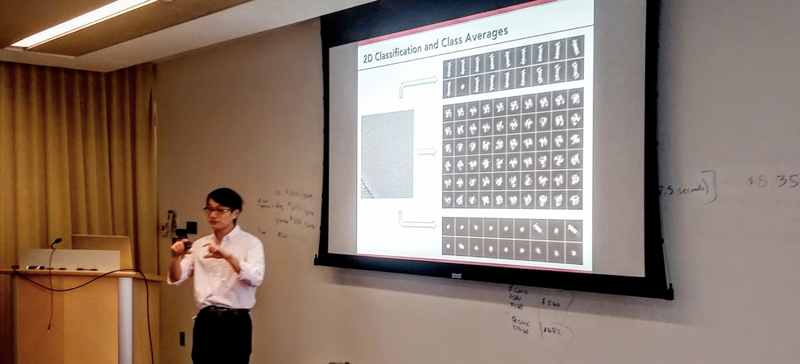
In the image processing step, you do unsupervised clustering of all of the different images of different molecules of your protein that you’ve obtained. Each one will be a 2D projection of the protein at a different angle, and there is no rhyme or reason — every rotation and orientation of the protein is equally likely. So by clustering, you can try to assemble a tumbling model, in essence stitching together cross-sectional data (separate images of different copies of the protein at different angles) into time series data (as if it was all images of the same molecule of the protein, tumbling in solution). You need hundreds or maybe thousands of images to do this.
The data you obtain are high dimensional. For instance, each image of a copy of the protein might be 300 x 300 pixels, which you can think of as a vector of 90,000 dimensions. Scientists therefore use standard dimensionality reduction tools such as principle components analysis (PCA) before trying to cluster the images.
After the unsupervised clustering step, you develop an initial model of what the protein structure might be. You then do supervised clustering of the images according to which angle of that initial 3D model they might correspond to. Then you have to go back and repeat the 2D clustering.
One problem with just using PCA for the 2D clustering, as described above, is that you don’t know where the mass center of the protein lies, and you don’t know rotation in the plane of view, so you don’t know how much two images might actually represent the exact same orientation of the protein, just translated or rotated in the xy plane. So on the second pass, after you’ve constructed an initial 3D model, you want to go back and do a more sophisticated 2D clustering. Two ways to determine 2D structure similarity that account for these issues are cross-correlation (which is noise-sensitive) and maximum-likelihood (which tolerates noise). In the maximum likelihood model, what you’re trying to maximize is the probability that a given 2D image was produced from a particular projection of your initial 3D model. You then cluster the 2D images based on which orientation they are most likely to correspond to.
The resolution of this technique depends on how good of 2D class averages (?) you can get. For this to be worth doing, at a minimum you need class averages good enough to yield 5 or 6Å resolution structures. With even better class averages you can get 3 or 4Å resolution structures. The theoretical limit of resolution of this technique is 1.8Å. So far this limit has only been approached for larger proteins (>90kDa), while for smaller proteins only 3Å structures have been obtained.
Note that because this is transmission electron microscopy, you actually see through the whole protein. So you can obtain high resolution even for interior sites of the protein, not just the surface. Note that you need some asymmetry in your protein in order to solve the protein’s structure. In the limit, if a protein had perfect radial symmetry, you wouldn’t be able to distinguish different sides of it at all.
All of this is only possible with direct detection (DD) cameras, which have only been available for about 2 years now.
You can inspect the Contrast Transfer Function (CTF) and Aberration of your images. CTF is the Fourier transform of the point spread function of the image. This essentially quantifies the amount of “defocus” of the microscope, a property which apparently is orthogonal to noise. It looks like a sine function, and everywhere that it crosses zero, you lose resolution. The solution is to collect images at multiple defocus levels and then apply the Wiener filter.
There are many tips and tricks, pitfalls, and various ways in which getting this to work for your protein can take some trial and error. Sometimes adding just a small amount of detergent to break surface tension can reduce the proportion of copies of your protein that “break” in the process of being pipetted onto the EM grid. Sometimes you have a protein complex where you can never get 100% purity of the whole complex — there are always some dissociated components of the complex in your field of view as well. And in general, no sample is 100% pure, and after you do 2D clustering on your images, you will need to throw out some fraction of the classes that simply do not correspond to the species you wanted to study.
For some examples, see structures of TRPV1 [Liao 2013], gamma secretase [Bai 2015], the inflammasome [Zhang & Chen 2015], and IDH1 bound to a small molecule ligand [Merk 2016]. Most of the highest-resolution structures have been obtained with 300 kV instruments, but Dr. Mao’s group at Harvard has been achieving comparable resolution with the 200 kV cryo-TEM Tecai Arctica. Indeed, there are still limitations in both protein preparation and computational analysis that prevent us from reaching the technical limitations of the equipment itself. Compute power can be limiting, and improvements in algorithms are continuing to improve resolution [Wu 2016].
Visit the IPCCSB website to learn more.

About Eric Vallabh Minikel
Eric Vallabh Minikel is on a lifelong quest to prevent prion disease. He is a scientist based at the Broad Institute of MIT and Harvard.