Estimation of penetrance using population allele frequency

Last month I was invited to speak at the Centers for Mendelian Genomics (CMG) Analysis and Methods Development meeting about “Population-based estimation of penetrance in rare disease”. Here is the blog post version of my talk.

what is penetrance and why do we care?

Penetrance is the probability of developing a particular disease given a particular genotype. One can speak of age-dependent penetrance, so the percentage of people with the genotype developing the disease by age 40, by age 50, and so on; I usually speak in terms of lifetime risk, meaning the probability that you ever develop the disease before you die. Inherent in this is that, for adult-onset diseases, lifetime risk can never quite be 100%, because you could always die of something else first.

Penetrance is hugely important for individuals undergoing predictive genetic testing — many people’s first question is, “does this mean I’ll definitely get the disease?”. Yet it is often very difficult to come by a firm estimate of penetrance.

traditional methods for estimating penetrance

In an ideal world, the right way to estimate penetrance would be to ascertain, from birth, a large cohort of people with a particular genotype, follow them until all have died of something or other, and then ask how many ever developed the disease before they died. Since genotyping technology was invented less than one human lifetime ago, this has never been done for any disease.

Instead, researchers often use family-based methods to estimate penetrance. A typical study would look at everyone who has been observed with the given genotype, and ask how many have diease, or how many have disease by a certain age. Family-based methods suffer from pervasive ascertainment bias [Minikel 2014]. Consider that some or all the following disclaimers usually apply to these studies:

• some individuals in the study have been ascertained on the basis of presenting with disease
• families in the study have been ascertained on the basis of having multiple affecteds
• the families originally used to establish that the variant causes the disease are included in the analysis
• not all unaffected individuals in the family have undergone predictive genetic testing

As an example of this last point, in genetic prion disease, only 23% of at-risk people choose predictive genetic testing [Owen 2014], and in pedigree data that I’ve had access to, we knew the genotypes of only 22% of at-risk individuals [Minikel 2014].

All of the factors listed above work in the same direction, tending to inflate one’s estimate of penetrance.

Researchers have been aware of these problems for a long time, and have proposed some solutions. As one example, the kin-cohort method [Wacholder 1998] involves ascertaining healthy individuals randomly from a population, genotyping them, taking a family history, and comparing survival curves of their first-degree relatives. This is a very clever solution, but it relies on being able to ascertain a large enough number of people with a disease-causing genotype without ascertaining on the presence of disease. So it worked for BRCA1 and BRCA2 variants in American Ashkenazi Jews [Wacholder 1998], but for many rarer genetic conditions, it’s impractical, because you would need to recruit tens or hundreds of thousands of people to find even one individual with a genotype of interest.

population-based methods

For all of the reasons described above, it’s very useful to have orthogonal, population-based methods, for asking questions about penetrance. The first key insight here is that a completely penetrant genetic variant should not be more common in the population than the disease that it causes. Applying this logic in practice means that you need good estimates of allele frequency even for uncommon variants, and that’s been hard to come by until recently. ExAC, a database of genetic variation in 60,706 human exomes, offers new opportunities [Lek 2016]. Many individuals in ExAC were ascertained as cases or controls for various common, complex diseases, but none were ascertained for Mendelian disease, so ExAC is a good reference database for studying most genetic diseases.

By providing allele frequency information in the general population, ExAC, like earlier reference databases such as ESP [Bell 2011, Xue 2012], has made it clear that clinical genetics has a big problem: many variants reported to cause genetic disease don’t actually cause genetic disease, or at least not most of the time.

Two databases — HGMD [Stenson 2014] and ClinVar [Landrum 2014] — collect assertions from the literature and from clinical labs stating that a particular genetic variant causes a particular genetic disease. At last count, there were over 100,000 unique reportedy disease-causing genetic variants in these databases. The average person in ExAC has 54 of them [Lek 2016]. Obviously, the average person doesn’t actually have 54 genetic diseases. Of course, much of this excess is caused by a small number of wildly high-frequency variants that obviously don’t cause any genetic disease, and much of it may be reportedly recessive variants found in a heterozygous state in ExAC. But even if we just look at variants in dominant disease genes at an allele frequency of <1%, we still see 0.89 reportedly pathogenic variants per person [Lek 2016], and it is clearly not the case that ~90% of people have a dominant genetic disease. So across the allele frequency spectrum, there are a lot of reportedly pathogenic variants that aren’t so pathogenic. When Anne O’Donnell and I looked at the reportedly pathogenic variants with the highest allele frequencies in ExAC, and asked how they had managed to be misclassified as pathogenic, we found that most of the time the problem traced to a paper in the literature that had made a claim of pathogenicity based on insufficient evidence.

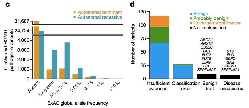
Above: Figures 3C and 3D from [Lek 2016]. Across the allele frequency spectrum and in both dominant and recessive disease genes, there are a lot of reportedly pathogenic variants that appear in ExAC. Of high (>1%) frequency reportedly pathogenic variants, a few are genuinely pathogenic, some are genuinely trait-associated but the trait is benign, and some are errors of annotation in databases — but the majority are based on literature with insufficient evidence.

Allele frequency information from ExAC has now enabled over 200 genetic variants to be reclassified from pathogenic to benign, likely benign, or of uncertain significance [Lek 2016, Whiffin & Minikel 2016]. These sorts of reclassifications sometimes trigger pushback from the original authors who proposed that a variant causes a genetic disease, who may argue that a variant could still be pathogenic, but with incomplete penetrance. But just how “incomplete” can incomplete penetrance be? We need to get quantitative, because if lifetime risk is at most 1%, then is it still reasonable to say that a variant “causes” a genetic disease, or is “pathogenic”? While allele frequency information can never prove that a variant has no association to disease, it can put bounds on what the possible penetrance might be, and in many cases, even for fairly rare variants, it is possible to show that there is no way a variant confers a level of risk anywhere remotely close to 100%.

To get quantitative, we need to extend our earlier observation — that a completely penetrant genetic variant should not be more common in the population than the disease that it causes. This is all simple math and population genetics, but it’s too often not applied in practice. Here are two ways we can think about allele frequency when making inferences about pathogenicity and penetrance.

1. maximum credible allele frequency

Say you’re studying the exome of a patient with Mendelian disease and trying to identify the causal variant. My colleague James Ware has devised a strategy for filtering that exome against the allele frequency information in ExAC, taking advantage of the following logic. The maximum allele frequency that is plausible for a variant to cause a dominant genetic disease is equal to the prevalence of the disease times the allelic heterogeneity (proportion of cases attributable to one variant) divided by penetrance (less penetrant variants can be more common), divided by 2 (because we are diploid):

For instance, prion disease causes in 1 in 5,000 deaths, and the most common variant (E200K) is found in 5% of cases [Minikel 2016], so a 100% penetrant variant cannot possibly have allele frequency greater than 0.0005% (1 in 200,000) [Minikel 2016]. Cardiomyopathy affects 1 in 500 people, the most common variant is found in <2% of cases, so a 50% penetrant variant cannot have an allele frequency greater than 0.004% [Whiffin & Minikel 2016]. The formula for recessive diseases is one notch more complicated but James has also worked it out and it is described in [Whiffin & Minikel 2016].

So whereas historically people have often filtered out variants with an allele frequency >0.1% when trying to identify the cause of a dominant disease [Bamshad 2011], we can actually be much more stringent. The caveat is that at low allele counts, our ability to estimate allele frequency is limited by sampling variance. For instance, if we look at variants seen at a 1% allele frequency among Europeans in ESP, these variants also have about a 1% frequency among ExAC Europeans. But variants with a 0.1% frequency in ESP tend to be slightly rarer in ExAC, and most singletons (variants seen exactly once in ESP) don’t reappear a second time in ExAC.

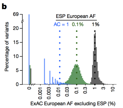
Above: Figure 3B from [Lek 2016]. The lower the allele count, the less good an estimate of allele frequency it provides.

Therefore, the lower the allele count, the more conservative we need to be. We’ve devised a framework for doing this using the 95% upper bound of the Poisson distribution on how many alleles might be observed at a given frequency, and have pre-computed values for all of ExAC (available on FTP) that you can use — read more about the methods in [Whiffin & Minikel 2016]. James has also created this handy web app that allows you to explore what the “maximum credible allele frequency” should be for your disease of interest.

Inherent in this approach is that the lower the penetrance of a variant, the higher frequency it might have in the general population. But you also have to figure that if penetrance is quite low, say, less than 10%, then the clinical utility of that variant is also low. James and Nicky Whiffin have presented data to show that almost all of the clinical utility of sequencing in cardiomyopathy comes from variants with a frequency of <0.001% — more common variants cumulatively contribute little, if any, risk [Whiffin & Minikel 2016].

2. estimation and bounds of lifetime risk

Remember that penetrance is the probability of disease given a particular genotype. Or, if we consider an allelic rather than genotypic model, the probability of disease given a particular allele. We can write this as P(D|A). Once we do, it becomes clear that, by Bayes’ theorem,

Each of these terms has a particular meaning:

• P(D|A) = penetrance
• P(D) = baseline risk (the lifetime risk of the disease in the general population)
• P(A|D) = allele frequency in cases
• P(A) = allele frequency in population controls

Note here that “population controls” means a group not selected for the presence, nor for the absence, of the disease. Just a slice of the general population.

So:

This logic is nothing new. The use of Bayes’ theorem to estimate disease risk dates back at least to the estimation of the risk of cancer in smokers [Cornfield 1951], and its application to genetics has been considered for almost as long [Li 1961]. But for this equation to work for rare diseases, you need pretty good estimates of case and population control allele frequency, and those have been hard to come by until recently. So thanks to ExAC, there are an increasing number of situations where this equation is relevant.

Here is the R code I’ve written (originally here) to estimate penetrance based on this formula.

library(binom)
penetrance = function(af_case, af_control, baseline_risk) {
  calculated_penetrance = af_case * baseline_risk / af_control
  estimated_penetrance = pmin(1,pmax(0,calculated_penetrance)) # trim to [0,1] support
  return (estimated_penetrance)
}
penetrance_confint = function (ac_case, n_case, ac_control, n_control, baseline_risk) {
  # for a genotypic model, use 1*n_case; for allelic, use 2*n_case
  case_confint = binom.confint(x=ac_case,n=2*n_case,method='wilson')
  control_confint = binom.confint(x=ac_control,n=2*n_control,method='wilson')
  lower_bound = penetrance(case_confint$lower,control_confint$upper,baseline_risk)
  best_estimate = penetrance(case_confint$mean,control_confint$mean,baseline_risk)
  upper_bound = penetrance(case_confint$upper,control_confint$lower,baseline_risk)
  return ( c(lower_bound, best_estimate, upper_bound) )
}

If you don’t want to run the R code yourself, James Ware has implemented it in the “penetrance” tab of this web app so you can just plug in your numbers into your browser.

In order to estimate 95% confidence intervals on penetrance, I’ve adopted the approach of [Kirov 2014]. You input the allele count (AC) and the number of individuals (N) for cases and controls, and the upper bound of the 95%CI is calculated based on the upper 95%CI of the binomial distribution for case allele frequency and the lower 95%CI for controls. Conversely, the lower bound of penetrance is based on the lower bound of case allele frequency and the upper bound of control allele frequency. You could rightly quibble that because this formula uses 95%CIs on both allele frequency values, the resulting confidence intervals are larger than they should be. You could also rightly quibble that the binomial distribution isn’t a good estimator at low allele counts, due to the bias illustrated in Figure 3B shown above (and I certainly would never apply this formula to singletons — variants observed only once in ExAC). But at the end of the day, for reasons I’ll discuss closer to the end of this post, this formula is really best used for obtaining a ballpark, order-of-magnitude estimate of penetrance. If you’re looking for an extremely precise point estimate of penetrance, this whole approach probably won’t work for you anyway.

If you rearrange the equation, another way to think about it is:

This means that the increased risk among people with a genotype is proportional to the ratio of case to population control allele frequency. So a variant that increases risk by 200-fold should be 200 times more common among cases than it is in the general population. (Note that this ratio of allele frequencies is slightly different than odds ratio although the two measures converge for very rare variants.)

application to prion disease

We walked through this logic in a study we published earlier this year, quantifying penetrance of prion disease variants [Minikel 2016, Markdown version here]. I care about prion disease for a personal reason — my wife harbors a pathogenic variant in PRNP — but it turns out that prion disease is also a great test case for using the above logic to estimate penetrance. None of the individuals in ExAC v1 were ascertained on neurodegenerative disease, so ExAC really is a good population control dataset for prion disease. And because prion diseases are “notifiable”, national surveillance centers have exceptionally good case ascertainment, and thanks to their generosity in sharing data, we were able to accumulate a dataset of 10,460 sequenced cases.

We found that the >60 variants reported to cause prion disease cumulatively have 52 alleles in ExAC. That means that almost 1 in 1,000 people has one of these variants, and thus, these variants are cumulatively much more common than all prion disease (which causes ~1 in every 5,000 deaths), let alone all genetic prion disease (only ~15% of cases are genetic). This is enough to tell us that not all of these variants can possibly be fully penetrant. In order to determine which variants were the culprits, we compared to the case series. Variants with excellent prior evidence of pathogenicity (Mendelian segregation and mouse models) were common in cases and absent from ExAC, consistent with complete or near-complete penetrance. Most of the excess allele count in ExAC was contributed by variants that were uncommon in cases and had weak prior evidence of pathogenicity — these variants are probably benign or contribute only a low risk. At least three variants appeared intermediate, as they were too common in controls for full penetrance, yet still enriched in cases over controls.

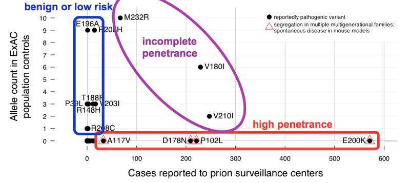
Above: an annotated version of Figure 2 from [Minikel 2016].

When we estimated penetrance for each variant, using the P(D|A) formula above, we found that there is a whole spectrum of penetrance for PRNP variants.

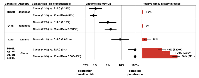
Above: Figure 3 from [Minikel 2016].

Note the scale on the x axis — for a disease so rare that the prior probability of developing it is only 0.02%, even a 50-fold increase in risk is only 1% lifetime risk. Reassuringly, the penetrance estimates that we derive from allele frequency information alone accord quite well with the proportion of cases that present with a positive family history.

This work has already led to a change in prognosis for some individuals who had originally been counseled that they were at risk for high-penetrance variants — see [Lebo 2016] and Erika Check Hayden’s article about ExAC. You can read out my and Sonia’s personal journey with this study here.

application to NR1H3

Multiple sclerosis (MS) is a complex disease with many genetic risk factors [IMSGC 2011], but no Mendelian form of the disease is known to exist. Earlier this year, a study reported that a missense variant in a nuclear hormone receptor — NR1H3 R415Q — causes the first-ever Mendelian form of MS [Wang 2016]. This claim was based on dominant segregation with disease in two families, but the LOD score was only 2.2 — below the threshold for genome-wide significance in family linkage studies, which is more like 3.0 or 3.6 [Lander & Kruglyak 1995, Kruglyak & Lander 1995]. And the variant in question has an allele frequency of 0.031% in ExAC non-Finnish Europeans. That may not sound like a high allele frequency, but it turns out to be way too high for this variant to cause Mendelian MS [Minikel & MacArthur 2016, full text here].

Consider that MS has a lifetime risk (in the general population) of 0.25% in women and 0.14% in men [Alonso & Hernan 2008]. If 0.06% of people in the general population are R415Q heterozygotes, and if even half them went on to develop MS, then this variant alone would account for 0.03% of the population developing MS. So if a total of 0.25% of people develop MS, then about 12% of them should have this variant. Instead, the variant was only found in 1 individual out of a case series of 2,053 MS patients [Wang 2016].

This works out to an allele frequency of 0.024% in cases, or 0.049% if we allow for 2 cases to be counted in the case series. This is not significantly higher than the frequency in ExAC. But if this variant causes MS, it should be more common in cases — much more common. Remember our rearranged formula earlier: P(D|A)/P(D) = P(A|D)/P(A). This means that if a variant increases risk by X-fold, it should be X times more common in controls. So if the baseline risk of MS is 0.25% and this variant is 50% penetrant, it should be 50/.25 = 200-fold more common in cases than controls. If it even had 10% penetrance, it should still be 10/.25 = 40 times more common in cases than in controls. Alternatively, you can think in terms of odds ratios instead of probabilities. The 0.25% lifetime risk in the general population means 1:399 odds, and if R415Q conferred 50% lifetime risk, that would be 50:50 odds. (50/50)/(1/399) = 399, so the odds ratio for R415Q would have to be 399 in order for this variant to have 50% penetrance.

Instead, if we apply our formula using the R code from earlier, assuming 0.25% baseline risk and basing the calculation on 2 alleles on 2,053 cases, versus 21 alleles in 33,369 ExAC individuals, we find that the upper bound of the 95%CI on penetrance is 2.2%. So even if R415Q were associated to MS risk, it couldn’t confer more than 2.2% lifetime risk of developing MS [Minikel & MacArthur 2016].

In their formal response [Wang 2016b] and in PubMed Commons the authors raised a comparison to LRRK2 G2019S in Parkinson’s disease, which everyone agrees is pathogenic, but which is also found in ExAC and has only a modest odds ratio, estimated at 9.6 [Do 2011]. For that variant, the math works out. Parkinson’s disease is at least an order of magnitude more prevalent than MS, with lifetime risk estimated anywhere from 3.7% [Elbaz 2002] to 6.7% [Driver 2009]. This order of magnitude greater prevalence means that the ~10-fold enrichment that has been observed — LRRK2 G2019S is found in roughly 0.1% of controls and 1% of cases [Gilks 2005, Do 2011] — is roughly consistent with the reported ~32% lifetime risk of Parkinson’s conferred by this variant [Ozelius 2006, Goldwurm 2007]. These quantitative details matter, and are different for every variant and every disease. That’s why the formulas discussed in this post are useful, even though they only provide very rough estimates and are subject to several caveats, as explained below.

caveats

In both of the applications described above, allele frequency information was used to get a rough estimate of penetrance. In prion disease, we were able to show that variants previously presumed highly penetrant conferred lifetime risk more on the order of 0.1%, 1%, or 10%. In the NR1H3 story, allele frequency information was sufficient to show that the reportedly causal variant couldn’t confer more than a few percent lifetime risk.

But trying to use allele frequency data to get a tighter estimate of penetrance would be very challenging. For instance, family-based studies have disagreed on the penetrance of PRNP E200K, with estimates ranging from 60% to 90% lifetime risk [Chapman 1994, Spudich 1995, D’Alessandro 1998, Mitrova & Belay 2002]. Since the prion study came out, I’ve had a few people from E200K families ask me whether ExAC data can help narrow down where the risk is within this range. The answer is, unfortunately, it can’t.

Here are the most important reasons why I think all penetrance estimates based on allele frequency need to be taken with a grain of salt:

• If a variant is highly penetrant, then it is hard to obtain a case series that doesn’t contain related individuals. If your case series has relateds, then technically you haven’t got an unbiased estimate of P(A|D).
• If a disease is fatal, then it is hard to obtain a population control series that isn’t at least somewhat depleted of people with variants that cause that disease. So then you don’t have an unbiased estimate of P(A) either.
• Comparisons of case and control allele frequency are vulnerable to confounding by population stratification. In the prion study, we didn’t have genome-wide SNP data on cases, so there was no way to perfectly control for this.
• Many causal variants for rare diseases are so rare that even with ExAC, we don’t yet have sufficiently precise estimates of allele frequency to give better than a rough answer.

With all that said, population-based allele frequency estimation is still a good way to get rough order-of-magnitude estimates of penetrance and to perform sanity checks on whether a genetic variant could plausibly be causal for a rare disease.