More on Convolutional Networks and Machine Learning
Last night I met up with @a in a Google+ hangout (by the way, an amazing tool– why do people still pay for GoToMeeting?), who talked me through the Turaga & Murray paper blogged about previously.
First, convolution. Convolution as these guys refer to it refers to applying kernels to an image, as in as this amazingly clear explanation. The process of machine learning is basically applying a bunch of these kernels serially as filters to the image, seeing how close you get to the desired segmentation, and then using backpropagation to modify the kernels (and some other parameters) to come closer to the desired segmentation the next time around.
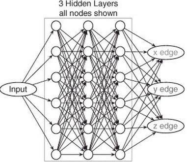
That’s the big picture, but the reality has some tricky notation to get a handle on. First, let’s understand how you move forward in the network, from input to output, given by Equation 2.1 and this helpful diagram:
Equation 2.1:
And here’s what I understand so far about the notation:
- For any given pair of nodes connected by an edge, the source node is subscripted as “b” and the destination node as “a”
- Ia is the image state at node a, and Ib is the image state at node b, i.e. after the convolution performed along the ba edge.
- ha is a bias applied at node a to all inputs received from all of its input nodes. This is just a scalar so it corresponds to a brightness offset (?). It lets you control how fast your program will converge on its final answer.
- wab is a kernel applied as a convolution on the edge from b to a, equivalent to one of the (simpler) kernels in the examples at aishack. Together, wab and ha are the things that get adjusted in this model as the machine learns.
- f(x) in Equation 2.1 is the sigmoid function: f(x) = (1 + e−x)−1 where x refers to a pixel, so you apply this function to each pixel x in the image to get the new value f(x) for each pixel
So the way to calculate Ia, i.e. to produce an image at each node a in the network, is as follows:
- For each input node b, convolute wab*Ib.
- Sum the results across all input nodes b
- Add the bias ha.
- Take the sigmoid function.
That’s how you move forward from input to output of the CN.
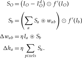
The magic of machine learning, though, is in the backpropagation algorithm. So you’ve moved forward, you got an output segmentation, and you scored it against a human-drawn ground truth to see how well it performed. Not very well. How will it learn to do better next time? That bit of skulduggery is given by:
Equation 2.2:
These equations describe how you change the parameters after you’ve got an output image from one iteration, in order to do better on the next iteration.
- IO is the output image you got
- IdO is the output image you desired
- f’(IO) is the derivative of the sigmoid function of IO.
- Circle with dot in the middle is pixel-wise multiplication
- SO, calculated from the above things, represents the difference between the desired and actual output image.
- Sa, represents the difference between desired and actual at each node a.
- Circle with star in the middle is cross-correlation.
- The second equation is telling you how to determine Sb from Sa, i.e. how to work backwards to find the good/badness of each node’s current settings, starting from the output node.
- η is a constant telling you by how much to change the gradient at each iteration.
- Cross-correlating ηIa with Sb gives you what the change to each kernel wab should be.
- Summing over all the pixels of Sa (multiplied by η) tells you what the change to the bias at that node should be.
All this has been immensely illuminating, but I have a lot of lingering questions to sort out. For one, I need to get a better handle on cross-correlation. Wikipedia’s explanation of cross-correlation has an EE spin to it, focused on signal processing, but for images the principles are the same, just with one extra dimension. You’re moving a small image around a large image looking for places where things match up. It asks the question, “where in this large image is this smaller image most nearly found?” Which leaves me with these questions:
- Ia and Sb should both be full-sized images (say, 1000×1000). How do you cross-correlate images of equal size? (I can imagine moving them around a few pixels and shaving off edges to see if one of them is just an xy translation of the other, but I’m not sure this is right)
- If they are both full-size images, their cross-correlation should also be 1000×1000. But then how can you assign the result of their cross-correlation as wab, which should have dimensions 5×5?
Then another question is about just how this backpropagation actually works. Apparently it’s all there in the above equations, which the authors follow with the statement “These equations implement an efficient recursive gradient computation that gives the backpropagation algorithm its name.” In order for this whole machine learning approach to move intelligently in the right direction and not just conduct an exhaustive search of the 10who knows how many possible combinations of kernels and biases, the program needs to know the derivative of its utility (how well its output will fit the final image) as a function of all its kernels and biases. I would have said there was no way to compute that derivative without just trying minute variations from one’s current position in a number of dimensions, but apparently those cross-correlations and pixel-wise multiplications actually compute that derivative.
To understand more about that I think my next move may be to read the LeCun papers that Turaga and Murray cite for their backpropagation algorithm:
While surfing around I also found source code for a CN implementation written by Alex Krizhevsky at University of Toronto. It’s in C#, whereas I was thinking of using Python both because I know it better and to stay more compatible with CellProfiler (though you could bridge through Cython I suppose?) but this might be a good reference to see how he implements things.


