QQ plots with matplotlib
After learning about QQ plots in last week’s post on genome-wide association studies, I got pretty excited about what a powerful tool these are. If you are making a huge number of statistical tests as is common in GWAS, QQ plots let you visualize (1) systematic biases (such as population stratification) and (2) whether the results of any of your tests might actually be significant. McCarthy 2008 and the paper he cites regarding QQ plots, Clayton 2005 both plot test statistics such as χ2 or Cochran-Armitage. But there’s no reason you can’t make a QQ plot directly with p values. Under the null hypothesis that none of the genotypes you’re looking at are actually associated with the phenotype you’re looking at, 5% of your tests should be significant at the .05 threshold, 1% at the .01 threshold, and so on. Why, that’s exactly what a p value means: “how likely was this result to have arisen under the null hypothesis?” Depending on the kind of data you’re working with, you might do an exact test where you directly compute a p value rather than a test statistic which you compare to a distribution. (For choosing a statistical test, the best reference I’ve found is John McDonald’s Handbook of Biological Statistics– particularly the choosing a statistical test page).
Today I wrote this Python script to generate a QQ plot using several of my favorite tools (all of which are open source). Psycopg interfaces Python to PostgreSQL, is dead easy to learn and I literally downloaded and installed it in less time than I’ve now spent writing this sentence. Numpy seems to be a favorite of scientists everywhere, and matplotlib is my new favorite visualization tool. What’s more, in case you were bored with the plain black text of code previously posted on this site, CureFFI.org now uses Pygments for syntax highlighting.
Here’s the code:
import sys
import math
import psycopg2 # http://www.initd.org/psycopg/
import numpy as np # http://numpy.scipy.org/
import matplotlib.pyplot as plt # http://matplotlib.sourceforge.net/

def generateqq():
    # get your already-calculated p values from PostgreSQL using psycopg
    conn = psycopg2.connect(database="mydb", user="postgres", password="password")
    conn.autocommit = True
    cur = conn.cursor()
    # retrive n, the total number of statistical tests made
    cur.execute("select count(*) n from test_p;")
    n = cur.fetchone()[0]
    print "n: ", n
    # retrive pmin, the most significant (i.e. min) p value (for defining the axes)
    cur.execute("select min(p_value) from test_p;")
    pmin = cur.fetchone()[0]
    print "pmin: ", pmin
    axisMax = math.ceil(-math.log10(pmin))
    print "axisMax: ", axisMax
    # calculate increment by which sorted p vals should increase under the null
    increment = 1.0/np.float64(n)
    print "increment: ", increment
    # starting value for series of 'expected' p values under null
    current_expected = np.float64(1.0)
    # lists for 'expected' and 'observed' p values
    expected = []
    observed = []
    counter = 0
    # retrive list of p values in descending order (least significant first)
    cur.execute("select p_value from test_p order by p_value desc;")
    for record in cur:
        expected.append(-math.log10(current_expected))
        observed.append(-math.log10(record[0]))
        current_expected -= increment
        counter += 1
        if (counter%100000 == 0):
            print "processed " + str(counter) + " rows" # so you don't get bored
    # now plot these two arrays against each other using matplotlib
    fig = plt.figure()
    plt.xlim([0,axisMax])
    plt.xlabel("Expected")
    plt.ylim([0,axisMax])
    plt.ylabel("Observed")
    plt.title("QQ Plot: Observed vs. Expected distribution of p values (-log10)")
    # the observed vs. expected data
    dataAx = fig.add_subplot(1,1,1)
    dataAx.plot(expected,observed,'r.') # red dots
    # a diagonal line for comparison
    lineAx = fig.add_subplot(1,1,1)
    lineAx.plot([0,axisMax],[0,axisMax],'b-') # blue line
    plt.show()
    # don't forget to close the database connection
    cur.close()
    conn.close()

if __name__ == '__main__':
    generateqq()
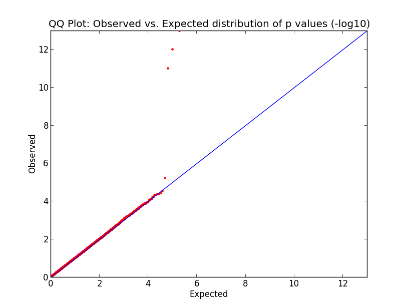
I tested it using made-up p values with this script. Here I add 200,000 random p values (simulating genes that aren’t significant) and 3 really small p values (simulating genes that are significant).
import sys
import math
import random
import psycopg2 # http://www.initd.org/psycopg/

conn = psycopg2.connect(database="mydb", user="postgres", password="password")
conn.autocommit = True
cur = conn.cursor()
for i in xrange(200000):
    cur.execute("insert into test_p(p_value) values (%s)",(random.random(),))
cur.execute("insert into test_p(p_value) values (%s)",(10e-12,))
cur.execute("insert into test_p(p_value) values (%s)",(10e-13,))
cur.execute("insert into test_p(p_value) values (%s)",(10e-14,))
cur.close()
conn.close()
Here’s what the output looks like:
What you’re looking at here in this simulation is pretty much what would happen in the GWAS of your dreams. The p values cling tightly to expectation (red dots along the blue line) for almost the entire domain, indicating that your data are good and unbiased, but just those last few p values are far above the line, indicating that you’ve found a few variants which are strongly correlated with phenotype. Hooray! Now let’s go translate these findings into therapeutic development.
Alas, these are made-up p values for this example. In reality you might see at least somewhat elevated p values across the domain, which could indicate a couple of things. Maybe you processed your cases in a different facility, at a different time, or under a different protocol than your controls, introducing systematic technical error. Or maybe your cases are related to each other (whether in a family or just in a broad ethnic group), so that some variants common to that family (or ethnic group) are enriched in cases and not in controls, even though those variants are not causally associated with the phenotype. But there are ways to address those issues, some of which are touched on in my recent GWAS post.

