PRNP deletions in 1000 Genomes are not real
One possible therapeutic strategy for prion diseases is to reduce or eliminate all PrP – that is, including healthy PrPC and not just diseased PrPSc. For instance, non-allele-specific gene therapy, or non-isoform-specific active immunization or passive immunization could target all PrP. Therefore it’s of great interest to know what the consequences of not having any PrP would be.
As reviewed in a recent post, mice [Bueler 1993], cows [Richt 2007] and goats [Benestad 2012] all survive without PrP. In fact, they seem quite healthy and have barely any phenotype at all under normal conditions [mice reviewed in Steele 2007]. Therefore it would be quite surprising if humans couldn’t survive without PrP. Still, we’ve never found someone without PrP, so our only evidence comes from these animal studies.
It was with great interest, then, that I noticed recently that dbVar contains an unvalidated report of a 4kb deletion covering all of PRNP exon 1, removing the transcription start site and all of the 5′UTR and presumably leading to no PRNP expression on the affected allele. This deletion was reported by the 1000 Genomes Project flagship paper [1000 Genomes Consortium 2010], in sample NA19238, a YRI female who is the mother in the Yoruban trio that was very deeply sequenced as part of the 1000 Genomes pilot. What’s more, NA19238 is suspected to also be the mother of NA18913, who is the father in a different trio [Roberson 2009, see Fig 6]. Though 1000 Genomes doesn’t have any phenotypic data per se, a putative grandmother would probably be of at least middle age and must obviously capable of the rigorous informed consent process of 1000 Genomes, effectively ruling out any dramatically shortened life or cognitive deficit. So even if this were just a hemizygous deletion of PRNP, it would be a lot more information than we have had so far about the phenotype of PRNP deletion in humans.
The fact that this would have been a big deal is your first clue that it might not be real. As Daniel MacArthur says:
The more interesting something is, the less likely it is to be real.
That’s just a bit of Bayesian reasoning: random errors in sequencing and variant calling are distributed uniformly across the genome, while prior probabilities of really shocking things like PRNP deletions are lower.
Still, it was worth looking into. My first step was to look at the underlying sequence data to see if it supported the existence of a deletion there, and since you can buy NA19238′s cell lines from Coriell I figured if it looked real we could Sanger sequence it.
First I wanted to know why this site was called as a deletion in the first place. I downloaded the list of variant calls from estd59 (the id for all the 1000 Genomes variants in dbVar) and grepped for essv271793 (the id of this particular deletion):
$ cat supporting_variants_for_estd59.csv | grep essv271793
"estd59","essv271793","CNV","Loss","","Sequencing","14","No","NA19238","None","","GRCh37 (hg19)","NC_000020.10","20","","","","","4665551","4669450","Remapped","1"
"estd59","essv271793","CNV","Loss","","Sequencing","14","No","NA19238","None","","NCBI36 (hg18)","NC_000020.9","20","","","","","4613551","4617450","Submitted Genomic",""
Of note: the ‘analysis ID’ is 14. Analysis 14 is defined here as:
Sequencing platform: Whole Genome Illumina. Mapping algorithm: MAQ. Type of computational approach: read depth analysis.
So this site was called as a deletion due to read depth. I downloaded the NA19238 BAMs from the 1000 Genomes pilot and used bedtools coverageBed to calculate coverage over the site of interest plus a couple of kb on either side (using the b36/hg18 base pair positions, and note use of -d to calculate depth at every individual base):
cat > delplus2kb.b36.bed
20 4611551 4619450
coverageBed -abam NA19238.chrom20.SLX.maq.SRP000032.2009_07.bam -b delplus2kb.b36.bed -d > NA19238.cov.del.b36
And then I pulled the coverage data into R and plotted it. Note that because R’s barplot() function does not keep the x axis true to scale, my code is a bit convoluted to get everything to line up.
cov = read.table("NA19238.cov.del.b36",col.names=c("chr","start","end","relpos","depth"))
xlab = "chr20:4611551-4619450"
ylab = "read depth"
main = "NA19238"
sub = "Site of proposed 3.9kb PRNP deletion"
bp_plotted = barplot(cov$depth,xlab=xlab,ylab=ylab,main=main,sub=sub) # capture the x axis spacing used by barplot()
falsezero=4611551 # position on chr20 where plot begins
# position of PRNP gene elements
prnp_tx=c(4615156,4630234) # FYI
prnp_exon1=c(4615156,4615382) # FYI
prnp_exon2=c(4627856,4630234) # FYI
# calculate range of PRNP transcript on barplot
prnp_tx_start_index = which(cov$relpos==4615156-falsezero)
prnp_tx_end_index = dim(cov)[1] #which(cov$relpos==4630234-falsezero) - beyond end of plot
prnp_tx_fixedx = bp_plotted[prnp_tx_start_index:prnp_tx_end_index]
# calculate range of PRNP exon 1 on plot
prnp_ex1_x = seq(4615156,4615382,10)
prnp_ex1_start_index = which(cov$relpos==4615156-falsezero)
prnp_ex1_end_index = which(cov$relpos==4615382-falsezero)
prnp_ex1_fixedx = bp_plotted[prnp_ex1_start_index:prnp_ex1_end_index]
# add PRNP exon 1 and transcript to plot
points(prnp_tx_fixedx,rep(1,length(prnp_tx_fixedx)),col="yellow",pch='.')
points(prnp_ex1_fixedx,rep(1,length(prnp_ex1_fixedx)),col="yellow",pch=15)
axis(side=1,at=bp_plotted)],lab=c("4611551","PRNP exon 1","PRNP intron 1","4619450"))
# calculate a smoothed 500bp running average of coverage - takes ~30 seconds
running_avg = vector(mode="numeric",length=dim(cov)[1])
for (i in 1:dim(cov)[1]) {
   running_avg[i] = mean(cov$depth[max(i-250,1):min(i+250,dim(cov)[1])])
}
# add the smoothed average to the plot.
points(bp_plotted,running_avg,col="red",pch='.')
With the result:

The black bars are the actual read depth, the red line is a smoothed 500bp rolling average, and the yellow represents PRNP gene elements. Sure enough, you can see a massive drop in read depth for about ~2kb right around PRNP exon 1. But I could also see two things that made me suspicious this might not be real. First, the dropoff in coverage is just a little bit too gradual – you can’t see clear breakpoints. Second, the average depth on either side of the deletion is about 20x, while the supposedly deleted area drops to ~5x. There’s always a lot of noise, of course, but a hemizygous deletion should drop by half, to ~10x, and a homozygous deletion should drop to ~0x, so this ~5x was pretty far from looking correct for either case.
If this were a real deletion, there should be informative traces of it in the sequence data besides just read depth. For instance, these libraries are paired-end 36bp reads with insert size of about 300, so you’d expect to find at least some read pairs that span the deletion and thus have an insert size of ~2000 in the BAM file. I used samtools view to slice out the reads from this range and sorted the TLEN field to find the largest inserts:
$ samtools view NA19238.chrom20.SLX.maq.SRP000032.2009_07.bam 20:4611551-4619450 | cut -f9 | sort -nr | head
476
464
456
455
450
448
441
440
440
439
$ samtools view NA19238.chrom20.SLX.maq.SRP000032.2009_07.bam 20:4611551-4619450 | cut -f9 | sort -nr | tail
-440
-440
-441
-446
-448
-450
-455
-456
-464
-476
No inserts larger than 500bp. Another sign that this deletion is not real. Still curious what was going on, I downloaded the BAMs for NA19238′s family members NA19239 and NA19240, and for the other deep trio from the 1000 Genomes pilot, the CEU (European Americans in Utah) trio of NA12891, NA12892 and NA12878. All six of them have more or less the same pattern at this site according to their SLX sequence data, but it’s somewhat less clear in SOLiD sequence data (available for two subjects, bottom row):

Now you can see how vanishingly unlikely this is seeming: a never-before-reported deletion that just happens to be present in all members of two trios, one European and one Yoruban. Much more likely to be a sequencing artifact.
But I was still curious why this particular sequencing artifact emerged. I went down the hall to ask my colleagues in the Talkowski Lab, who are experts in calling structural variants from sequence data. They agreed this didn’t look like a real deletion, and Ian Blumenthal suggested I try looking at the Mapability track in the UCSC Genome Browser. That track captures some of the variation in sequence depth due to non-uniqueness of sequence across the genome. While I was fiddling around in the genome browser I noticed a track for GC Percent and turned that on as well:
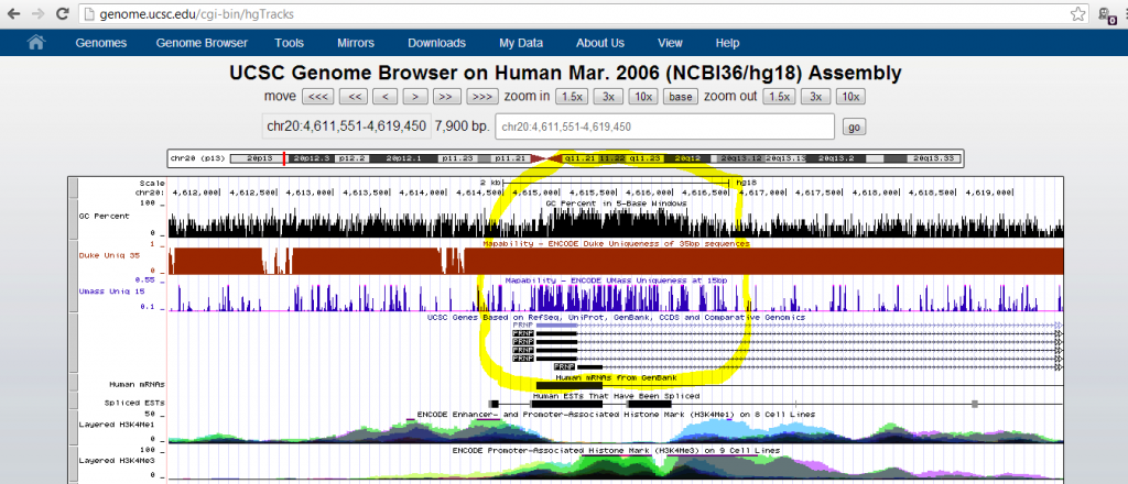
Mapability (blue above) turned out to be pretty decent at this site, but GC content (black) was quite elevated. I recalled that at the UAB sequencing course last year, Shawn Levy introduced some of the difficulties with GC content. The higher the GC content, the more thermally stable the DNA, so it doesn’t melt as well and is poorly amplified with PCR. Therefore high-GC genomic regions tend to be underrepresented in sequence data, and this problem is especially bad if you start with only small amount of input DNA and then do a lot of PCR cycles (see also PCR duplicates).
I clicked View > DNA in the Genome Browser to get the reference sequence at this site, removed the line endings and then read the file into R to calculate a rolling average of GC content that I could mash up with my read depth plot:
# read in a text file with the DNA bases for this 8kb region on one line
dna=read.table("DNA-20-4611551-4619450-stripped.txt")
d =as.character(dna$V1[1]) # convert from factor to string
dnabases=substring(d, seq(1,nchar(d),1), seq(1,nchar(d),1)) # adapted from http://stackoverflow.com/questions/2247045/r-chopping-a-string-into-a-vector-of-character-elements
# calculate a rolling 500bp average of gc content
gc=vector(mode="numeric",length=length(dnabases))
for (i in 1:length(dnabases)) {
   gc[i] = mean(dnabases[max(i-250,1):min(i+250,length(dnabases))]%in%c('G','C'))
}
gc = gc[1:dim(cov)[1]] # cleave off the last base - incompatibility in 0- vs. 1-based numbering
points(bp_plotted,gc*40,col="purple",pch='.') # plot the GC content
axis(side=4,at=seq(0,40,4),lab=seq(0,1,.1)) # add an axis for GC content
mtext(text="GC content",side=4) # label the axis
And there it was, a smoking gun:
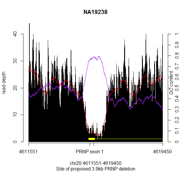
GC content (purple) is hugely elevated at exactly the site where the read depth (red) is depleted. They match up almost perfectly.
I asked my colleague Vamsee Pillalamarri in the Talkowski Lab if he could check one of his datasets at the same site, and he sent me back this read depth plot from one of the samples he’s currently working on:

He has zero coverage at the exact same site as the deletion was called in NA19238. There you have it: after all this, it’s just a GC content issue. Glad I decided to look at the sequencing reads before ordering the cells and Sangering them!
update 2013-04-01: While I was doing this analysis I noticed that dbVar also contains a call of a nearby 1Mb deletion covering PRNP and several other genes in NA12891, reported by the same study as the above deletion. Such a very large deletion seems even less likely than the 4kb NA19238 deletion above, but I figured while I’m at it and have the NA12891 BAMs on hand anyway I might as well check.
First I checked what analysis had led to this variant call:
$ cat supporting_variants_for_estd59.csv | grep essv274112
"estd59","essv274112","CNV","Loss","","Sequencing","19","No","NA12891","None","","GRCh37 (hg19)","NC_000020.10","20","","","4082925","5007416","4082755","5007606","Remapped","1"
"estd59","essv274112","CNV","Loss","","Sequencing","19","No","NA12891","None","","NCBI36 (hg18)","NC_000020.9","20","","","4030925","4955416","4030755","4955606","Submitted Genomic",""
Analysis 19 is read pair mapping using mrFAST:
Sequencing platform: Whole Genome Illumina. Mapping algorithm: mrFAST. Type of computational approach: read pair mapping.
Again, as I’ve reasoned above, a true deletion should show itself in more than one way. Though this ‘deletion’ may have been called based on aberrant read pairs, if it’s real it should also result in reduced read depth. It doesn’t. I created a bed file with three elements, one for the deletion and one each for the 1Mb before and after it, and calculated coverage using coverageBed -hist:
$ cat > NA12891.del.b36.bed # the 1 Mb before and after the deletion too
20 3030755 4030755
20 4030755 4955606
20 4955606 5955606
$ coverageBed -abam NA12891.chrom20.SLX.maq.SRP000032.2009_07.bam -b NA12891.del.b36.bed -hist> NA12891del.cov.b36.hist
Result: average read depth is 33.1 for 1Mb before the ‘deletion, 34.8 in the ‘deletion’ and 35.4 for 1 Mb after the ‘deletion’. I didn’t bother to take the time to figure out what mrFAST had actually seen as aberrant in NA12891 – it might well represent a real inversion or translocation, but those wouldn’t affect PRNP transcription. Based on the read depth we can pretty well rule out a true deletion.

About Eric Vallabh Minikel
Eric Vallabh Minikel is on a lifelong quest to prevent prion disease. He is a scientist based at the Broad Institute of MIT and Harvard.