Histone marks at 5' vs. 3' ends of genes: a gentle slope or sudden dropoff?
Today at work a discussion came up about histone modifications vs. position within a gene, particularly with regards to H3K9 acetylation. H3K9ac is an activating epigenetic marker – it is associated with increased levels of transcription and is thought to opens up chromatin, making it easier for RNA polymerase to get in and transcribe. Levels of H3L9 acetylation are generally higher at the 5′ (start) of a transcript than at the 3′ (end) of a transcript. Wikipedia even says, “H3K9ac is found in actively transcribed promoters” – i.e. 5′ ends. Our director Jim Gusella asked the question, does H3K9 acetylation gently slope off across the length of the gene, or is it a sudden dropoff? Marcy MacDonald asked the same question of H3K36me3, which is another activating mark but one which is generally associated with “actively transcribed gene bodies” rather than just promoters.
It occurred to me we should be able to answer these questions using ENCODE data. ENCODE has done hundreds of genome-wide ChIP-seq experiments, pulling down various histone modifications (or transcription factors, etc.) and asking what parts of genomic DNA they were bound to.
So I looked up the available ENCODE data for these two histone marks. There was only one cell line, NT2-D1, in which both H3K9ac and H3K36me3 have been measured. NT2-D1 is a “malignant pluripotent embryonal carcinoma”. (Sadly they did not do transcription level or RNA polymerase in this cell line, otherwise it would be interesting to throw that in as well). I grabbed the “Signal” (note: not “Peak”) data for these two histone marks from the UCSC Table Browser like so:
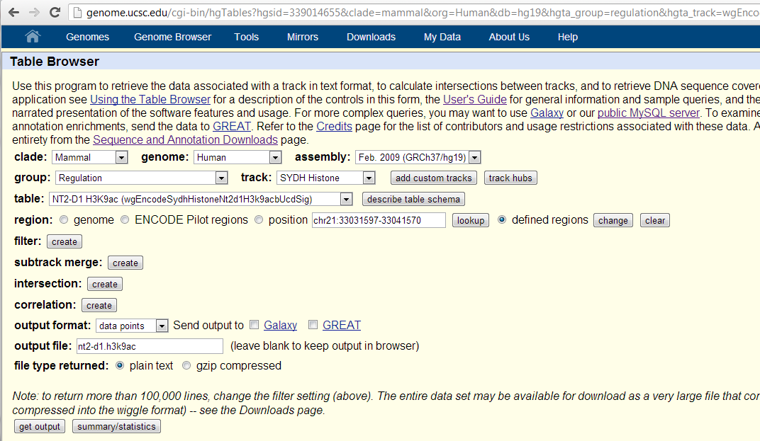
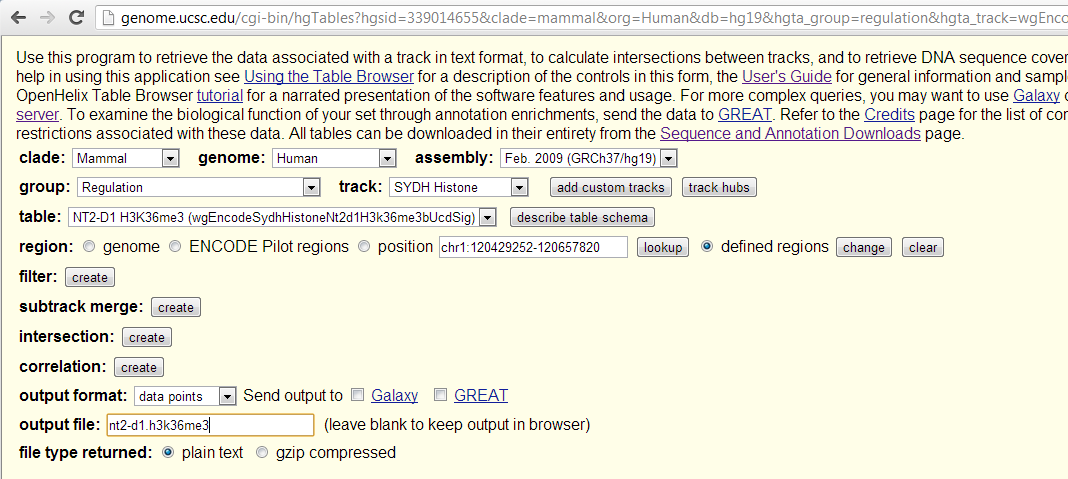
Note that I used the ‘defined regions’ option and pasted in BED formatted list of the start and stop positions of RefSeq transcripts of my two favorite genes, HTT (chr4) and PRNP (chr20), as examples to play with:
chr4	3076407	3245687
chr20	4666796	4682234
Then I wrote this quick R script to process the raw data I got out and turn it into some plots.
setwd('c:/sci/026rplcl/data/ref/')

h3k36me3 = read.table('nt2-d1.h3k36me3',skip=2)
h3k9ac = read.table('nt2-d1.h3k9ac',skip=2)

colnames(h3k36me3) = c('chr','startb','endb','depth')
colnames(h3k9ac) = c('chr','startb','endb','depth')

# add gene names to the tables. note this lazy method only works if you are looking at <= 1 gene per chromosome
matchgene = data.frame(c('chr4','chr20'),c('HTT','PRNP'),c('+','+'))
colnames(matchgene) = c('chr','gene','strand')

h3k36me3 = merge(h3k36me3,matchgene,by='chr')
h3k9ac = merge(h3k9ac,matchgene,by='chr')

for (geneid in matchgene$gene) {
  png(paste(geneid,'.png',sep=''))
  temp1 = subset(h3k36me3, gene==geneid) # get data for current gene of interest
  temp1 = temp1[with(temp1,order(startb)),] # make sure it's in order by base pair position
  temp2 = subset(h3k9ac, gene==geneid)
  temp2 = temp2[with(temp2,order(startb)),]
  ylim = c(0,max(c(temp1$depth,temp2$depth)))
  plot(temp1$startb,temp1$depth,pch=19,type='l',lwd=2,col='orange',ylim=ylim,xlab='bp',ylab='sequence depth',main=geneid) # plot H3K36me3
  points(temp2$startb,temp2$depth,pch=19,type='l',lwd=2,col='blue',ylim=ylim,xlab='bp',ylab='sequence depth',main=geneid) # plot H3K9ac
  if (matchgene$strand[matchgene$gene==geneid] == '-') { # add the 3' and 5' labels
    axis(side=1,pos=0,at=c(min(temp1$startb),max(temp1$startb)),labels=c("3'","5'"),lwd=0)
  } else if (matchgene$strand[matchgene$gene==geneid] == '+') {
    axis(side=1,pos=0,at=c(min(temp1$startb),max(temp1$startb)),labels=c("5'","3'"),lwd=0)
  }
  legend('topright',c('H3K36me3','H3K9ac'),col=c('orange','blue'),pch=15,cex=1.5)
  dev.off()
}
matchgene = data.frame(c('chr4','chr20'),c('HTT','PRNP'),c('+','+'))
colnames(matchgene) = c('chr','gene','strand')
h3k36me3 = merge(h3k36me3,matchgene,by='chr')
h3k9ac = merge(h3k9ac,matchgene,by='chr')
for (geneid in matchgene$gene) {
png(paste(geneid,'.png',sep=''))
temp1 = subset(h3k36me3, gene==geneid) # get data for current gene of interest
temp1 = temp1[with(temp1,order(startb)),] # make sure it's in order by base pair position
temp2 = subset(h3k9ac, gene==geneid)
temp2 = temp2[with(temp2,order(startb)),]
ylim = c(0,max(c(temp1$depth,temp2$depth)))
plot(temp1$startb,temp1$depth,pch=19,type='l',lwd=2,col='orange',ylim=ylim,xlab='bp',ylab='sequence depth',main=geneid) # plot H3K36me3
points(temp2$startb,temp2$depth,pch=19,type='l',lwd=2,col='blue',ylim=ylim,xlab='bp',ylab='sequence depth',main=geneid) # plot H3K9ac
if (matchgene$strand[matchgene$gene==geneid] == '-') { # add the 3' and 5' labels
axis(side=1,pos=0,at=c(min(temp1$startb),max(temp1$startb)),labels=c("3'","5'"),lwd=0)
} else if (matchgene$strand[matchgene$gene==geneid] == '+') {
axis(side=1,pos=0,at=c(min(temp1$startb),max(temp1$startb)),labels=c("5'","3'"),lwd=0)
}
legend('topright',c('H3K36me3','H3K9ac'),col=c('orange','blue'),pch=15,cex=1.5)
dev.off()
}
And here’s the result:


A couple of things jump out from at least these two examples:
- H3K9ac is a sharp dropoff – it’s high right in the promoter and then drops off quickly to very little enrichment for the rest of the gene
- H3K36me3 is more consistent throughout the gene, and appears to maybe be slightly more enriched towards the 3′
Both of the enrichment profiles are pretty jagged, and I’m not clear on whether that reflects actual differences in enrichment levels across the gene, or sequencing artifacts (GC content, alignability, etc.).

About Eric Vallabh Minikel
Eric Vallabh Minikel is on a lifelong quest to prevent prion disease. He is a scientist based at the Broad Institute of MIT and Harvard.