Properties of CNS drugs vs. all FDA-approved drugs

motivation

Armed with my new list of FDA-approved drugs and annotation as to which are CNS drugs, I set out to characterize the chemical space of CNS drugs as another exercise to learn a bit of cheminformatics.

I didn’t address this in my last post, but the method I used for defining CNS drugs basically amounts to whether they are licensed for a CNS indication. This isn’t a perfect proxy for blood brain barrier permeability, which is the property I am really interested in. There are false negatives – plenty of drugs cross the blood-brain barrier yet aren’t licensed for any CNS-related purpose (say, simvastatin). Emily Ricq pointed out there might also be false positives – drugs with a CNS indication that actually stay in the periphery and act in trans, though I haven’t found an example yet. And of course, my list probably isn’t complete. Still, my hope is that this list of CNS drugs might provide a pretty decent outline of what chemical space BBB-permeable drugs tend to occupy.

background & setup

To do this, I set out to calculate a number of properties of each of the drugs on my list – CNS and otherwise – and then plot and examine the ranges of different properties along with some principal components.

As Rajarshi Guha pointed out last time, there’s no need to include every imaginable descriptor, and just using a handful of key physicochemical properties can be enough for a good analysis.

In casting around for a list of properties to start from, I noticed each ZINC catalog entry also has a link for “Properties”, a small tab-delimited text file (the extension is .xls but they’re not actually Excel files) with the ZINC id, SMILES and nine physicochemical properties. These are defined in the ZINC paper [Irwin & Stoichet 2005] Here’s what each of those properties means:

MWT: molecular weight.
LogP: partition coefficient, a measure of relative solubility in a hydrophobic vs. hydrophilic solvent, usually octanol and water. True logP must be determined empirically, but can be predicted computationally by several different methods. According to [Irwin & Stoichet 2005] the values in ZINC are predicted using the fragment-based method employed by molinspiration [Ertl 2000] and are similar to xLogP by [Wang 1997].
Desolv_apolar: apolar desolvation energy (kcal/mol). There weren’t any really good web resources on this concept – the best I could find was this. It appears to be the energy required to remove solvent from the compound, i.e. the reduction in free energy achieved by dissolving the compound. In this case, the solvent is assumed to be apolar.
Desolv_polar: apolar desolvation energy (kcal/mol). Presumably same as above but with a polar solvent.
HBD: number of hydrogen bond donors (i.e. parts willing to be the positively charged or H side of a putative hydrogen bond). According to Lipinski’s Rule of Five a drug ought to have no more than five.
HBA: number of hydrogen bond acceptors (i.e. parts willing to be the negatively charged side of a putative hydrogen bond). According to Lipinski’s Rule of Five a drug ought to have no more than ten.
tPSA: topological polar surface area. A measure of polarity and of hydrophilicity. tPSA is a major determinant of blood brain barrier penetrance; Armin Giese has cited a rule of thumb that this should be < 80 or 90 Å² for a drug to penetrate the CNS.
Charge: net charge of the molecule
NRB: number of rotatable bonds. This describes the conformational flexibility of the molecule and is also a determinant of drug-likeness and oral bioavailability. A non-standard variant of Lipinski’s Rule of Five holds that a drug ought to have fewer than ten rotatable bonds [Veber 2002].

In addition, the ZINC paper also lists several other properties which don’t appear in the downloadable Properties files but which nevertheless sound important [Irwin & Stoichet 2005]:

number of chiral centers
number of chiral double bonds (E/Z isomerism)
number of rigid fragments

Unfortunately not all of these items appear to be available in the list of CDK descriptors. The relevant descriptors I was able to find are:

Weight.MW
XLogP.XLogP*
TPSA.TopoPSA
HBondAcceptorCount.nHBAcc
HBondDonorCount.nHBDon
RotatableBondsCount.nRotB

Weirdly, net charge is not one of the available descriptors, but this is trivial to calculate from SMILES: total number of + minus total number of -. Still this leaves me without the desolvation energies, number of chiral carbons and double bonds, and number of rigid fragments. If anyone has ideas of how to get these, let me know.

Then there’s the matter of which logP prediction algorithm to use. As noted above, ZINC’s method is most similar to xLogP. I was at first put off from using XLogP.XLogP because calling this descriptor on aminophylline threw a null pointer exception (minimum script to reproduce error). I tried using ALogP.ALogP instead, but this often (38 = 2.2% of 1691 FDA-approved drugs) returns NA values, which I would need some way to handle for principal components analysis. Then I read this excellent post by Rajarshi Guha ground-truthing different logP prediction algorithms, which stated that aLogP was vastly inferior to xLogP. So finally I returned to xLogP and just threw out molecules that caused errors, using the same try-catch logic I was using to skip unparseable SMILES strings.

In the end, here’s the code I wound up with:

setwd('c:/sci/037cinf/analysis/1')
options(stringsAsFactors=FALSE)
library(stringr)
library(rcdk)

# /wp-content/uploads/2013/10/drugs.txt
fda_drugs = read.table('c:/sci/037cinf/analysis/1/drugs.txt',sep='\t',header=TRUE)

# get list of molecular descriptors, minus #28 IPLearning which makes R hang
descriptors = get.desc.names(type='all')[-28]

# note these indices are _after_ eliminating the original item #28
descriptors_to_use = descriptors # respectively HBA, HBD, NRB, TPSA, MWT, XLOGP
compounds = data.frame(id=integer(),name=character(),cpdset=character(),smiles=character(),
                       hba=integer(),hbd=integer(),nrb=integer(),
                       tpsa=numeric(),mwt=numeric(),xlogp=numeric(),
                       charge=integer())
starttime = Sys.time()
for (i in 1:dim(fda_drugs)[1]) {
  if (fda_drugs$smiles[i] == "") { next }
  # try catch logic from http://stackoverflow.com/questions/8093914/skip-to-next-value-of-loop-upon-error-in-r-trycatch
  parse_smiles_error = tryCatch ( 
    { cpd_object = parse.smiles(fda_drugs$smiles[i]) },
    error = function(e) e
  )
  if(inherits(parse_smiles_error,"error")) next
  id = i
  name = fda_drugs$generic_name[i]
  if(fda_drugs$cns_drug[i]) {
    cpdset = 'fda_cns'
  } else {
    cpdset = 'fda_non_cns'
  }
  smiles = fda_drugs$smiles[i]
  hba = eval.desc(cpd_object, descriptors_to_use[1])
  hbd = eval.desc(cpd_object, descriptors_to_use[2])
  nrb = eval.desc(cpd_object, descriptors_to_use[3])
  tpsa = eval.desc(cpd_object, descriptors_to_use[4])
  mwt = eval.desc(cpd_object, descriptors_to_use[5])
  xlogp_error = tryCatch( 
    # throws null pointer exception on aminophylline
    { xlogp = eval.desc(cpd_object, descriptors_to_use[6]) },
    error = function(e) e
  )
  if(inherits(xlogp_error,"error")) next # just skip any molecules that throw null pointed exceptions on xlogp
  # tried this, now discarded: # alogp = eval.desc(cpd_object, descriptors_to_use[7])[1]
  nplus = str_count(smiles,"[+]") # + is not a metacharacter inside [] in POSIX regular expressions, see http://farazmahmood.wordpress.com/2008/11/10/regular-expression-escaping-meta-characters-within-character-classes/
  nminus = str_count(smiles,"[-]")
  charge = nplus - nminus
  named_row = cbind(id,name,cpdset,smiles,hba,hbd,nrb,tpsa,mwt,xlogp,charge)
  rownames(named_row) = id
  compounds = rbind(compounds,named_row)
}
elapsed = Sys.time() - starttime
elapsed
colnames(compounds) = c("id","name","cpdset","smiles","hba","hbd","nrb","tpsa","mwt","xlogp","charge")

analysis

I began by plotting the molecular weight vs. xLogP:

plot(compounds$mwt, compounds$xlogp, pch=19, col='#999999',
     xlab='MWT',ylab='XLogP',main='CNS vs. all FDA-approved drugs, MWT and XLogP')
points(compounds$mwt[compounds$cpdset=='fda_cns'], compounds$xlogp[compounds$cpdset=='fda_cns'],pch=19,col='orange')
legend('bottomleft',c('All FDA-approved drugs','CNS drugs'),col=c('#999999','orange'),pch=19,cex=.8)

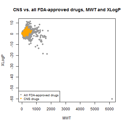
A single outlier has totally dominated the range of the plot. Here’s where I’m glad I went to all that effort to have a table that matches common names to SMILES. I can now ask, what is that thing?

compounds[compounds$mwt > 6000,]

It turns out to be inulin – not insulin, but a different thing. It’s a large sugary biomolecule used for monitoring kidney function. Mind you, insulin would be twice as large again, at ~12 kDa. But insulin, like most of the biologicals, was implicitly filtered out because DrugBank stores an amino acid sequence, not a SMILES string, for it, so I never parsed it and included it in the analysis. There are plenty of therapeutic antibodies yet much larger than insulin and none of those are here either. Since we’re not being exhaustive regardless, I decided to exclude inulin from the rest of the analysis to focus on the true small molecules. With it gone, here’s what the plot looks like:

inulin = compounds$mwt > 6000
plot(compounds$mwt[!inulin], compounds$xlogp[!inulin], pch=19, col='#999999',
     xlab='MWT',ylab='XLogP',main='CNS vs. all FDA-approved drugs, MWT and XLogP')
points(compounds$mwt[compounds$cpdset=='fda_cns'], compounds$xlogp[compounds$cpdset=='fda_cns'],pch=19,col='orange')
legend('bottomleft',c('All FDA-approved drugs','CNS drugs'),col=c('#999999','orange'),pch=19,cex=.8)

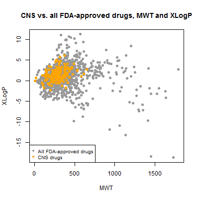
Now we can see that virtually all CNS drugs have a molecular weight less than about 600 Da and an xLogP between about 5 and -5. Interesting that they’re of moderate xLogP in the scheme of all drugs – one often hears of CNS drugs needing to be relatively hydrophobic, but they aren’t the most extreme hydrophobes either. But though I call this “moderate”, the range here is quite considerable when you remember that logP is the log of the ratio of concentration in octanol vs. water. So a logP of 5 means there is 10⁵ as much of the molecule in the octanol as in the water, and -5 means the converse. That’s a big difference.

Among the non-CNS drugs, the spread is even starker – a few drugs have 10¹⁰ the concentration in octanol as in water, and vice versa. I wondered which drugs these are and what they look like.

# from /2013/09/23/a-quick-intro-to-chemical-informatics-in-r/
rcdkplot = function(molecule,width=500,height=500,...) {
  #par(mar=c(0,0,0,0)) # set margins to zero since this isn't a real plot
  temp1 = view.image.2d(molecule,width,height) # get Java representation into an image matrix. set number of pixels you want horiz and vertical
  plot(NA,NA,xlim=c(1,10),ylim=c(1,10),xaxt='n',yaxt='n',xlab='',ylab='',...) # create an empty plot
  rasterImage(temp1,1,1,10,10) # boundaries of raster: xmin, ymin, xmax, ymax. here i set them equal to plot boundaries
}

par(mfrow=c(2,3))
for (i in which(compounds$xlogp > 10)) {
  rcdkplot(parse.smiles(compounds$smiles[i])[[1]],main=compounds$name[i])
}

Here are the most hydrophobic drugs, with the most octanol-favoring partition coefficient:

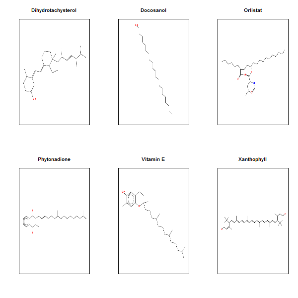
They’re almost pure hydrocarbon, with only an O or two here and there. And the most hydrophilic drugs:

par(mfrow=c(2,2))
for (i in which(compounds$xlogp < -10)) {
  if (i %in% c(586,604,608)) next # skip one that throws an error - "Molecule must be connected"
  rcdkplot(parse.smiles(compounds$smiles[i])[[1]],main=compounds$name[i])
}

And here are the most hydrophilic ones:

These are almost completely coated in polarizable heteroatoms.

Next I plotted tPSA vs. xLogP. I would expect these to be correlated and they are, though the correlation is a bit noisier than I might have thought:

plot(compounds$tpsa[!inulin], compounds$xlogp[!inulin], pch=19, col='#999999',
     xlab='tPSA',ylab='XLogP',main='CNS vs. all FDA-approved drugs, tPSA and XLogP')
points(compounds$tpsa[compounds$cpdset=='fda_cns'], compounds$xlogp[compounds$cpdset=='fda_cns'],pch=19,col='orange')
abline(v=90,col='red')
legend('bottomleft',c('All FDA-approved drugs','CNS drugs'),col=c('#999999','orange'),pch=19,cex=.8)

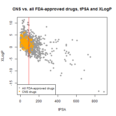
The CNS drugs certainly skew towards lower tPSA, though ~12% of them are above the 90 Å² threshold cited here and 3% (6 out of 221) are above the looser 120 Å² mentioned here. Some of these might be false positives – nominally CNS drugs that aren’t actually BBB-permeable. For instance, the highest tPSA was 136.22 Å² for meloxicam, an NSAID. I didn’t find any data on BBB permeability but it has been investigated as a treatment for traumatic brain injury, where it has been suggested to help BBB integrity [Hakan 2010]. This could potentially be a proper CNS indication that doesn’t actually involve crossing the BBB itself.

Next I looked at hydrogen bond donors vs. acceptors. Since both relate to size, I’d expect a correlation, and indeed, they have a Pearson’s correlation of .91.

plot(compounds$hba[!inulin], compounds$hbd[!inulin], pch=19, col='#999999',
     xlab='HBA',ylab='HBD',main='CNS vs. all FDA-approved drugs, HBA and HBD')
points(compounds$hba[compounds$cpdset=='fda_cns'], compounds$hbd[compounds$cpdset=='fda_cns'],pch=19,col='orange')
legend('bottomright',c('All FDA-approved drugs','CNS drugs'),col=c('#999999','orange'),pch=19,cex=.8)

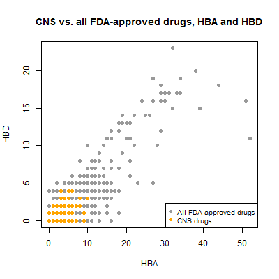
Recall that Lipinski’s Rule of Five suggests that drugs for any indication should have ≤ 5 hydrogen bond donors and ≤ 10 hydrogen bond acceptors. Many of the non-CNS drugs violate this guideline, but all of the CNS drugs obey it.

Molecular weight and number of rotational bonds were also highly correlated, with a Pearson’s of .83:

plot(compounds$mwt[!inulin], compounds$nrb[!inulin], pch=19, col='#999999',
     xlab='MWT',ylab='NRB',main='CNS vs. all FDA-approved drugs, MWT and NRB')
points(compounds$mwt[compounds$cpdset=='fda_cns'], compounds$nrb[compounds$cpdset=='fda_cns'],pch=19,col='orange')
legend('bottomright',c('All FDA-approved drugs','CNS drugs'),col=c('#999999','orange'),pch=19,cex=.8)

And one more surprise – though almost all CNS drugs (and all drugs generally) are neutral, a handful of CNS drugs (7 of them) do actually have a net charge:

barplot(table(compounds$charge[compounds$cpdset=='fda_cns']),col='orange',xlab='charge',ylab='frequency',main='Charge of CNS drugs')

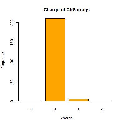
This list includes lithium (Li⁺) of course, as well as GABA. Now, I’m not sure how much stock to put in these charge figures since charge depends for instance on the pH you’re assuming the molecule is at and therefore whether acids are protonated or not. I know that ZINC uses a SMILES string chosen to represent a realistic state somewhere in pH 5 – 9.5 [Irwin & Stoichet 2005] but I didn’t find any info on how DrugBank chooses the protonation state of molecules that it represents in the SMILES strings.

Finally, I did a quick principal components analysis. There are only a few descriptors here anyway, but I was still a bit surprised that the first two PCs explain 99.97% of variance; the other PCs didn’t seem worth looking at.

compounds_ni = compounds[!inulin,]

cpd_mat = as.matrix(compounds_ni[,5:11])
covmatrix = cov(cpd_mat) # calculate covariance matrix
eig = eigen(covmatrix) 
pc = cpd_mat %*% eig$vectors 

plot(pc[,1],pc[,2],pch=19,col='#999999',xlab='PC1 (94.7%)',ylab='PC2 (5.3%)',
     main = 'PC1 vs. PC2 of FDA-approved drugs')
points(pc[compounds_ni$cpdset=='fda_cns',1],pc[compounds_ni$cpdset=='fda_cns',2],pch=19,col='orange')
legend('bottomright',c('All FDA-approved drugs','CNS drugs'),col=c('#999999','orange'),pch=19,cex=.8)

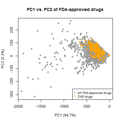
And again, the CNS drugs cluster together, occupying a considerably smaller chemical space than the set of all approved drugs. This is all well-known information. It’s exciting for me that I was able to reproduce this result with this simple dataset.