A quick intro to chemical informatics in R
Today my colleague Emily Ricq introduced me to the amazing world of chemical informatics, a whole field I didn’t know existed. We were discussing the various high throughput screens that have been done to discover anti-prion compounds, and what sorts of interesting meta-analysis could be done on them. As one example, she pointed me to a paper [Singh 2009] which compared the properties of molecules found in four different chemical libraries.
The authors did several types of analysis, one of which I’ll talk briefly about here. First they generated a bunch of different features or “descriptors” for each molecule. A descriptor can be any property of the molecule, from trivial stuff like molecular weight and charge to slightly more esoteric properties like clogP to yet fancier stuff I don’t begin to understand. Then they did a principal components analysis on the molecules and then scatterplotted the molecules in each library versus the set of FDA-approved drugs [Fig 5]. I was surprised by how little the two clouds of points overlapped: most of the molecules in these libraries occupy a chemical space quite distant from the approved drugs. That’s bad news for anyone hoping to find therapeutic hits in those libraries and then develop them into a drug.
This seemed like a simple analysis I could wrap my head around, so to get my feet wet in this world of chemical informatics I decided it would be interesting to see whether a few of my favorite antiprion compounds fall within the space of approved drugs or not. This post walks through the analysis I did.
getting started
Rajarshi Guha (also a co-author on the Singh 2009 paper) has written a couple of awesome chemical informatics packages for R entitled rcdk and rpubchem [Guha 2007]. I used rcdk and it was shockingly easy to get set up with. The functionality is implemented in Java and this is an R interface to it, so you also need rJava. I already had that, so I just loaded the rcdk package which takes several minutes – it’s huge.
install.packages("rcdk") # huge, takes a few mins to download
library(rcdk) # docs at http://cran.r-project.org/web/packages/rcdk/rcdk.pdf, paper at http://www.jstatsoft.org/v18/i05/paper
Next I sought to manually create a Java object for a molecule from its SMILES. SMILES is a systematic, unambiguous plain-text representation of molecular structure. I found anle138b‘s SMILES in its PubChem entry. For many molecules you can also find them on Wikipedia.
# parse.smiles accepts a vector of SMILES strings and returns a list of type AtomContainer,
# containing items of type IAtomContainer
# if you have just one molecule of interest, just grab the first item with [[1]]
anle138b = parse.smiles("C1OC2=C(O1)C=C(C=C2)C3=CC(=NN3)C4=CC(=CC=C4)Br")[[1]]
The next thing I wanted to do is plot it. The draw.molecule.2d function draws it in a separate Java window:
# draws it in a separate Java window
view.molecule.2d(anle138b)
That function is especially nice because if you pass it multiple molecules it can plot them all in a grid for comparison. But for just one molecule I thought it would be nicer to plot directly in R, so adapting a bit of code from the rcdk docs I wrote this function:
rcdkplot = function(molecule,width=500,height=500) {
    par(mar=c(0,0,0,0)) # set margins to zero since this isn't a real plot
    temp1 = view.image.2d(molecule,width,height) # get Java representation into an image matrix. set number of pixels you want horiz and vertical
    plot(NA,NA,xlim=c(1,10),ylim=c(1,10),xaxt='n',yaxt='n',xlab='',ylab='') # create an empty plot
    rasterImage(temp1,1,1,10,10) # boundaries of raster: xmin, ymin, xmax, ymax. here i set them equal to plot boundaries
}
And when I call it on anle138b, sure enough, that’s the molecule I know:
rcdkplot(anle138b)

Cool. Now when I went to do the same for one of my other favorite antiprion compounds, curcumin, I realized how lame it is that R has no way to read literal strings ignoring escape sequences. Python has this with r"" for instance mystring=r"string with a backslash (\) in it", but R has no equivalent. Thus there’s no way to make this work:
curcumin = parse.smiles("O=C(\C=C\c1ccc(O)c(OC)c1)CC(=O)\C=C\c2cc(OC)c(O)cc2")[[1]] # won't work
..without going in and manually changing all the single backslashes to double backslashes:
curcumin = parse.smiles("O=C(\\C=C\\c1ccc(O)c(OC)c1)CC(=O)\\C=C\\c2cc(OC)c(O)cc2")[[1]] # will work, but it's a pain to manually edit
Which is a pain to do. In practice this probably only comes up when you’re just trying to do a simple demo of something, like I was; if you actually had a real analysis to do you would probably be reading your dataset from disk, in which case read.table with allowEscapes=FALSE would do the trick.
The next thing I learned about rcdk is how to get these descriptors of molecules. rcdk comes with access to a whole list of descriptors which you can get like so:
descriptors = get.desc.names(type="all")
This gave me a vector of character strings, the names of fifty descriptors you can calculate on your molecule. I figured a good one to try out would be the number of strikes a molecule has against it as a drug according to the Rule of Five:
# get one descriptor, for instance Rule of Five descriptors http://en.wikipedia.org/wiki/Lipinski's_rule_of_five
eval.desc(anle138b,"org.openscience.cdk.qsar.descriptors.molecular.RuleOfFiveDescriptor")
Hooray – anle138b has zero failures, i.e. it complies with all of the tenets of the Rule of Five. You can also get some properties of a molecule using rcdk’s base functions, like get.total.charge, get.volume, get.exact.mass, etc.
Now, to do something more interesting I needed a database of chemicals. I quickly discovered ZINC, UCSF’s public database of all things chemical biology: molecules, their properties, which compound libraries they’re found in. It’s fantastically easy to browse or download data in a variety of formats. Coming from the world of bioinformatics, I was amazed at how utterly the cheminformatics people are pwning us at the open data game.
For starters I looked up MSDI’s US Drug Collection, the set of 1,280 FDA-approved drugs that was used in one recent anti-prion screen [Karapetyan & Sferrazza 2013]. ZINC is so awesome that can actually generate for you a shell script you can use to download the data for this library (see links at bottom of this page). I downloaded the US Drug Collection in SDF (structure-data file) format:
wget http://zinc.docking.org/db/byvendor/msusdrugs/usual.sdf.csh
csh usual.sdf.csh
gunzip *.gz
Then read them into R:
msdi_usdrugs = load.molecules(c("msusdrugs_p0.0.sdf","msusdrugs_p1.0.sdf"))
length(msdi_usdrugs)
# [1] 2319
Now, one thing that’s confusing – I still haven’t figured out why the SDF files contain 2319 compounds even though the library is only supposed to be 1280. And there is no metadata with common names (e.g. drug names), etc. which might be nice to have. (If you know the deal, please leave me a comment!)
Anyway, setting that issue aside for a moment, I set out to have rcdk calculate descriptors on these 2319 molecules for me. (Although, by the way, the most important properties can be downloaded directly from ZINC – see the “Properties” link on each chemical library’s page, for instance, this link).
The rcdk paper [Guha 2007] has code for looping through a chemical library and calculating descriptors on each molecule. But when I tried to use it, I discovered that R would hang on the first molecule. By trial and error I figured out that of the 50 descriptors in rcdk, number 28, entitled "org.openscience.cdk.qsar.descriptors.molecular.IPMolecularLearningDescriptor" was making it hang. So I eliminated that one:
descriptors = get.desc.names(type="all")
# eliminate #28, "org.openscience.cdk.qsar.descriptors.molecular.IPMolecularLearningDescriptor"
# because it is so compute-intensive it makes R hang
descriptors = descriptors[-28]
And with that I could calculate all the other descriptors. But it took over 10 seconds per molecule. I didn’t want to wait all day, and plus most of the descriptors are highly correlated with each other anyway and I’m not doing any fancy analysis here, just getting my feet wet. So I wrote a quick loop to identify which descriptors were taking so long:
times = numeric(length(descriptors))
for (j in 1:length(descriptors)) {
   start_time = Sys.time()
   eval.desc(msdi_usdrugs[[1]], descriptors[j]) # calculate descriptor j
   times[j] = as.numeric(Sys.time() - start_time) # figure out how long that just took. i'm assuming all will be in seconds.
}
sum(times > .05) # only 14 of the 49 take > .05 second
descriptors_to_use = descriptors[-which(times > .05)] # eliminate the descriptors that take > .1 second to calculate
And found that only 14 of the 49 remaining descriptors took more than .05 seconds each, so I removed those (last line above). With that, I was able to do all the other descriptors for all 2319 compounds in just 33 minutes, again using code modified from Guha’s rcdk paper:
# remove all the repeated parts from the descriptor names - code from the rcdk paper
desc_names = gsub("org.openscience.cdk.qsar.descriptors.molecular.","", descriptors_to_use)
desc_names = gsub("Descriptor","", desc_names)

desc.list = list() # initialize a list
col_names = c() # initialize column names
start_time = Sys.time() # start time
for (i in 1:length(msdi_usdrugs)) {  # loop through molecules
    tmp = c() # a running list of all sub-descriptors for this molecule
    for (j in 1:length(descriptors_to_use)) {  # loop through descriptors
        values = eval.desc(msdi_usdrugs[[i]], descriptors_to_use[j]) # calculate descriptor - each one returns a vector
        tmp = c(tmp, values) # add the vector to the running list
        if (i == 1) # only on the first iteration, come up with column names
            col_names = c(col_names, paste(desc_names[j], names(values), sep='.'))
        }
    desc.list[[i]] = tmp # add the sub-descriptor values to the master list
}
desc.data = as.data.frame(do.call("rbind", desc.list)) # convert to data frame
names(desc.data) = col_names # assign column names

execution_time = Sys.time() - start_time # see how long that took
To make things interesting, I also wanted to compare at least a few antiprion compounds from the literature, so I chose anle138b, cpd-B and IND24, the three most potent compounds in vivo:
antiprion_cpds = parse.smiles(c(
    "CC1=CC=CC(NC2=NC(C(C=C3)=CC=C3C4=CC=CC=C4)=CS2)=N1", # IND24, a 2-aminothiazole
    "C1(C2=CC=C(N/N=C\\C3=CC=NC=C3)C=C2)=CN=CO1", # cpd-B. note double backslash to escape
    "C1OC2=C(O1)C=C(C=C2)C3=CC(=NN3)C4=CC(=CC=C4)Br" # anle138b
))
And I re-ran the above loop with these three compounds instead of the MSDI US Drug Collection, and concatenated the results to the bottom of the original data frame:
desc.list = list() # initialize a list
col_names = c() # initialize column names
start_time = Sys.time() # start time
for (i in 1:length(antiprion_cpds)) {  # loop through molecules
    tmp = c() # a running list of all sub-descriptors for this molecule
    for (j in 1:length(descriptors_to_use)) {  # loop through descriptors
        values = eval.desc(antiprion_cpds[[i]], descriptors_to_use[j]) # calculate descriptor - each one returns a vector
        tmp = c(tmp, values) # add the vector to the running list
        if (i == 1) # only on the first iteration, come up with column names
            col_names = c(col_names, paste(desc_names[j], names(values), sep='.'))
        }
    desc.list[[i]] = tmp # add the sub-descriptor values to the master list
}
desc.data2 = as.data.frame(do.call("rbind", desc.list)) # convert to data frame
names(desc.data2) = col_names # assign column names
desc.data.all = rbind(desc.data,desc.data2)
With the data in hand for the FDA-approved drugs plus antiprion compounds, I wanted to do a principal components analysis, which I usually do “manually” following this tutorial. The matrix contains NaN values, which there is really no good way to handle. Most of the NaN were concentrated in a few rows (i.e. a few molecules) so I thought about just removing those with desc.mat.no.na = desc.mat[-which(rowSums(is.na(desc.mat)) > 0),] but I didn’t want to remove what might have been precisely the most interesting molecules for all I knew. So I just converted NaN to zero.
desc.mat = matrix(unlist(desc.data.all), ncol=134, byrow=TRUE) # convert to matrix. thanks to http://stackoverflow.com/questions/13224553/how-to-convert-a-list-to-a-matrix-more-efficiently-in-r
desc.mat.no.na = desc.mat
desc.mat.no.na[is.na(desc.mat)] = 0
covmatrix = cov(desc.mat.no.na) # calculate covariance matrix
eig = eigen(covmatrix)
pc = desc.mat.no.na %*% eig$vectors # multiply matrices to get principal components# eig = eigen(covmatrix)
dim(pc) # 2322  134
Next I plotted the proportion of variance explained by the first 50 PCs:
plot(1:50,(eig$values/sum(eig$values))[1:50],pch=19, ylim=c(0,1), xlab='PC#', ylab='Variance explained', main='Variance explained by PCs')
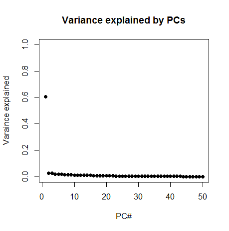
Whoa! PC1 explains about 60% of variance. That one looks important. Now, a great many of the descriptors I had generated were simply quantities of things found in the molecule – for instance, there are 20 columns that just represent the number of each of the 20 canonical amino acids found in the molecule. And there are columns for weight and number of hydrogen bond acceptors, etc. Therefore I had a strong hunch that PC1 might simply be representing the size of the molecule. So I browsed the list of column names and found that column 27, "AtomCount.nAtom" is simply the number of atoms in the molecule. And sure enough, PC1 is very strongly correlated with this, rho = -.83.
> cor.test(pc[,1],desc.mat.no.na[,27])

        Pearson's product-moment correlation

data:  pc[, 1] and desc.mat.no.na[, 27]
t = -72.6193, df = 2320, p-value < 2.2e-16
alternative hypothesis: true correlation is not equal to 0
95 percent confidence interval:
 -0.8453742 -0.8204896
sample estimates:
       cor
-0.8333537
And PC1 is similarly correlated with column 130, the molecular weight (rho = -.66).
OK, so PC1 has to do with size of the molecule. And note the correlation is negative, so higher PC1 is lower molecular weight. Here’s a plot of PC1 vs. PC2:
var.exp = (eig$values/sum(eig$values))
plot(pc[,1],pc[,2],pch=16,xlab=paste("PC1 (",formatC(var.exp[1]*100,digits=1,format="f"),"%)",sep=""),ylab=paste("PC2 (",formatC(var.exp[2]*100,digits=1,format="f"),"%)",sep=""),main="PC1 vs. PC2 of US Drug Collection")
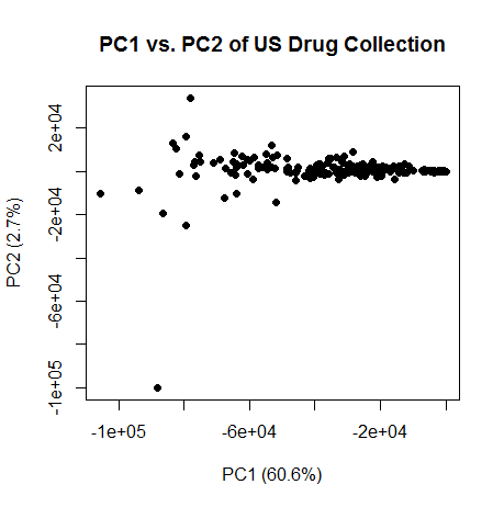
The smaller molecules are on the right, larger on the left. Curiously, PC2 really only has two very extreme outliers, and everything else falls in a narrow line. What on earth is PC2 capturing? I remembered hearing somewhere that after size, hydrophobicity is the next biggest explainer of variance in molecular properties. Sure enough, I discovered that PC2 is somewhat correlated (rho = -.11, p = 8e-8) with column 1, "ALOGP.ALogP", a measure of hydrophobicity (see partition coefficient) and with column 4, "APol.apol", a measure of polarity (rho = -.17, p < 2e-16). So PC2 might be measuring something to do with hydrophobicity. But I’d hesitate to assign much significance to this yet – hydrophobicity might be correlated with size, for instance, and since PCs are orthogonal to each other, PC2 would have to at best represent the component of hydrophobicity that isn’t explained by size. In any case, these are PCs of a bunch of metrics most of which I don’t understand very well.
Now for the interesting part. I read in Singh 2009 that chemical libraries are full of compounds that look nothing at all like a drug – to the point that even in the first few principal components they fail to overlap with the drugs. Is that true of these 3 antiprion compounds?
plot(pc[,1],pc[,2],pch=16,xlab=paste("PC1 (",formatC(var.exp[1]*100,digits=1,format="f"),"%)",sep=""),ylab=paste("PC2 (",formatC(var.exp[2]*100,digits=1,format="f"),"%)",sep=""),main="PC1 vs. PC2 of US Drug Collection")
legend("bottomright",c("FDA-approved drugs","antiprion compounds"),col=c("black","orange"),pch=16,cex=.8)
points(pc[2320:2322,1],pc[2320:2322,2],col='orange',pch=16)
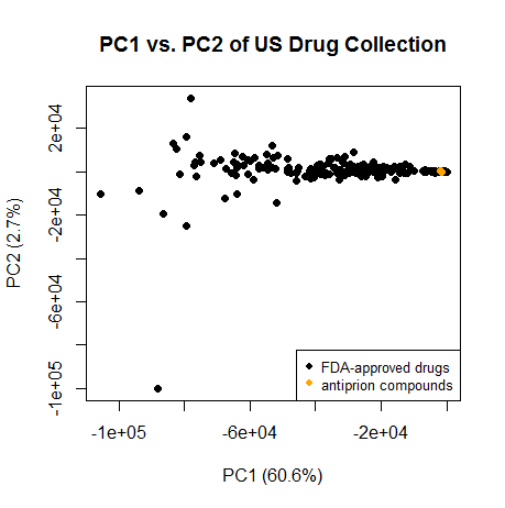
No – in fact, in the first 2 PCs they cluster quite cleanly with the FDA-approved drugs. They’re towards the right, meaning they’re on the small size for a drug, which makes sense given that (unlike many drugs) they need to be able to cross the blood-brain barrier. And on whatever dimension PC2 is measuring, they’re also squarely in the mode.
Same on PC2 and PC3:
plot(pc[,2],pc[,3],pch=16,xlab=paste("PC2 (",formatC(var.exp[2]*100,digits=1,format="f"),"%)",sep=""),ylab=paste("PC3 (",formatC(var.exp[3]*100,digits=1,format="f"),"%)",sep=""),main="PC2 vs. PC3 of US Drug Collection")
legend("bottomright",c("FDA-approved drugs","antiprion compounds"),col=c("black","orange"),pch=16,cex=.8)
points(pc[2320:2322,2],pc[2320:2322,3],col='orange',pch=16)
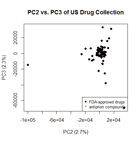
Again, they cluster squarely with most of the drugs.
None of this analysis is too meaningful because these PCs depend on what descriptors were included in the first place, and I didn’t understand enough of them to make meaningful choices. For instance, perhaps by throwing out all the descriptors that took a long time to calculate I eliminated a lot of the really interesting metrics. Or perhaps I should have pruned the glut of boring descriptors related to a molecule’s size, and then PC1 wouldn’t be quite so dominant at 60.6% of variance.
Once I iron out some kinks like which descriptors to use (and ideally figure out some better way of handling NaN values), what I’d like to do eventually is get the full list of antiprion compounds in SMILES form and see how they cluster in the principal component space. According to Emily Ricq, sometimes you can see discrete clusters in PC space for different mechanisms. On reflection that’s exactly what I’d expect for anti-prion compounds. The small planar aromatic molecules like anle138b, cpd-B and IND24, quinacrine, chlorpromazine, etc. which interfere with prion conversion but don’t necessarily bind PrP monomers all fall into one pretty tight cluster, and the long anionic polymers like heterpolyanion-23, dextran sulfate, pentosan polysulfate, antisense oligonucleotides, etc. which do bind PrP should all fall into another distinct cluster. It would be interesting to see if there are any other clusters as well. Where would curcumin and amphotericin b fall?
So far I’m quite impressed with the cheminformatics world. I learned tools, found relevant data and wrote this whole post in just several hours, something I would consider unthinkable for a newcomer to bioinformatics. I’m hopeful that with some more tinkering I’ll be able to start learning some interesting stuff about anti-prion molecules.

About Eric Vallabh Minikel
Eric Vallabh Minikel is on a lifelong quest to prevent prion disease. He is a scientist based at the Broad Institute of MIT and Harvard.