Why a simple exponential model of prion kinetics in vivo won't work
In a recent post I explored the kinetic models of prion propagation in cell culture, walking through the logic of [Ghaemmaghami 2007] and showing why the simplest model isn’t sufficient to explain observed results. Here I want to do the same thing for in vivo prion replication.
model
I’ll assume that degradation of PrPSc follows first-order kinetics, consistent with the data from [Safar 2005b] and the assumptions in [Ghaemmaghami 2007].
Based on the “heterodimer model” in which 1 PrPC + 1 PrPSc → 2 PrPSc, I’ll assume a rate law in which the production rate of PrPSc is proportional to both [PrPC] and [PrPSc]. Note that this implicitly assumes that all PrPSc is capable of converting PrPC and thus amounts to equating PrPSc with infectivity, which is an assumption I’ll carry throughout this model. If you’re not comfortable with this assumption, stay tuned – we’ll talk about it lots more below.
Here I’m modeling the situation in the brain, where we’re primarily talking about post-mitotic cells and, in any event, even the cells that do divide don’t increase in number over one’s lifetime, so cell division does not come into play, unlike in my earlier post.
The change in PrPSc is production minus degradation, so:
PrP^{Sc}(t) - k_{degradation}PrP^{Sc}(t)")
I’ll use S(t) to refer to [PrPC] as a function of time, and T(t) to refer to PrPSc as a function of time. So:
T(t) - k_{degradation}T(t)")
Rearranging we have:
(k_{conversion}S(t) - k_{degradation})")
Now I’ll assume that the expression level of PrPC, denoted S(t), does not change as a function of time. This isn’t quite correct – see PrPC downregulation – and we’ll talk more about that later. For now, I’m building a simple model, so let’s say that a given animal has expression level S0 and that S(t) = S0 for all t.
(k_{conversion}S_0 - k_{degradation})")
The solution to this differential equation is:
 = T_0 e^{(k_{conversion}S_0 - k_{degradation})t}")
Observe that this describes an unstable system which has but one steady state, where:

In other words, a steady state level of PrPSc can be maintained only if conversion and degradation are perfectly balanced. If the system tips just slightly off of this steady state, then PrPSc will either be degraded to nothing or will replicate exponentially without bound. In [Ghaemmaghami 2007] this sort of system was rejected on the basis of experimental evidence: more than one steady state had been observed in cell culture. But here we can’t reject this system outright because in vivo, no steady state has ever been observed – prion infection of the CNS leads inevitably to death. (There have been some claims of stable “subclinical” prion infection, but I’m not convinced by any of these – see points 3 and 4 in my post on PrPL).
However, in this post I’m going to use a different line of reasoning to argue why simplified system described above can’t be an accurate model in vivo.
the data
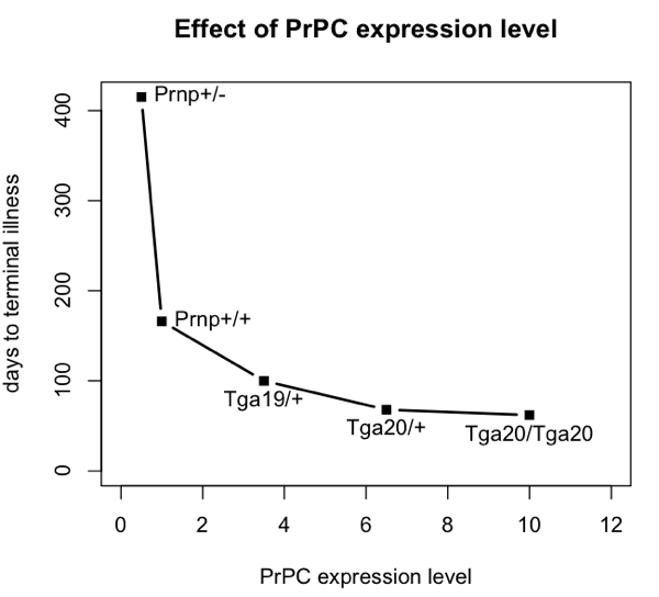
To do this, I’m going to base my argument on the incubation times for prion disease in intracerebrally inoculated mice with different levels of PrPC expression. Here are data from Fischer 1996 (ft) Table 1:
| mouse genotype name | PrPC expression level (relative to wild-type) |
days to onset of symptoms | days to terminal illness |
|---|---|---|---|
| Prnp+/- | 0.5 | 290 | 415 |
| Prnp+/+ | 1.0 | 131 | 166 |
| Tga19/+ | 3.5 | 87 | 100 |
| Tga20/+ | 6.5 | 64 | 68 |
| Tga20/Tga20 | 10 | 60 | 62 |
Here’s a plot of those data:
mousename = c("Prnp+/-","Prnp+/+","Tga19/+","Tga20/+","Tga20/Tga20")
explevel = c(.5,1,3.5,6.5,10) # PrPC expression level
symptoms = c(290,131,87,64,60) # time to symptoms
terminal = c(415,166,100,68,62) # time to terminal illness
plot(explevel,terminal,type='b',pch=15,lwd=2,xlim=c(0,12),xlab='PrPC expression level',ylab='days to terminal illness',ylim=c(0,max(terminal)),main='Effect of PrPC expression level')
text(explevel,terminal,labels=mousename,pos=c(4,4,1,1,1))
All of these mice were i.c. inoculated with the same dose of prions – 30 μL of a 1% brain homogenate, apparently following the same methods as in [Bueler 1993]. The number of median infectious doses (ID50s) inoculated is never explicitly calculated in either paper, but I can hazard a guess. Bueler’s mice contained 8.1 log10 ID50s at terminal illness, so if a brain is about 1 mL, then 30 μL of a 1% brain homomgenate is about log10(108.1 * (.030/100)) = 4.6 log10 ID50s. In any event, the exact number isn’t important, just the fact that they were all inoculated with the same dose.
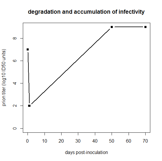
But the inoculated dose isn’t necessarily the dose that’s relevant as a starting point for modeling prion replication. As stated in Prusiner 1982:
After intracerebral inoculation of hamsters with 107 ID50 (median infectious dose) units, about 102 ID50 units can be recovered in the brain 24 hours later. During the next 50 days the amount of agent in the brain increases to 109 ID50 units. At this time the agent is widely distributed throughout the brain and no regional differences are apparent. The neuropathology is minimal and the animals exhibit no neurological dysfunction… By 60 to 70 days, vacuolation of neurons and astrogliosis are found throughout the brain, even though the titer of the agent remained constant.
Prusiner is referring to hamsters, while Fischer’s data are from mice, so ignore the exact numbers of days on the x axis, but basically what Prusiner is sketching out is this:
days = c(0,1,50,70)
logtiter = c(7,2,9,9)
plot(days,logtiter,type='b',ylim=c(0,9),xlab='days post-inoculation',ylab='prion titer (log10 ID50 units)',pch=15,main='degradation and accumulation of infectivity',lwd=2)
For that first day, clearly something is going on which we’re not going to be able to capture in this model. One possibility is that for the first day, PrPSc is by far the excess reactant locally at the inoculation site, such that 99.999% of it gets degraded without managing to convert any PrPC. The tiny amount of PrPC that does get locally converted in that first 24 hours is what then goes on to spread and infect the rest of the brain. This may not be the right explanation, though. Because prion strains appear to follow their own neurotropic patterns rather than preferentially killing the neurons adjacent to the inoculation site, it seems likely that prions spread in three dimensions through the brain very quickly relative to the total time of the incubation period. Indeed, some very old literature seems to support that: Bueler 1993 cites Millson 1979, who found that infectivity was widely distributed across the entire periphery within 30 minutes after i.c. infection, though different brain regions were not examined. (Bueler also cites two other studies, Cairns 1950 and Hotchin 1983, but neither of these relates to i.c. inoculation of scrapie). I’m not sure that one study by Millson really settles it, but since I haven’t modeled the three-dimensional spread of prions anyway, perhaps for this model it’s simplest to assume instant distribution of prions throughout the brain, and argue that the reason PrPSc is the excess reactant is that some other limited resource is saturated for those first few days. We’ll talk more about saturation later on in this post.
I’m not sure exactly where infectivity hits its nadir, but Bueler 1993 reports that after inoculation of wild-type mice with 7.0 log10 ID50s, only 1.5 log10 ID50s remained in the brain 4 days after inoculation. So I’ll assume that the starting titer – T0 in my notation – is 1.5 log10 ID50, and I’ll assume that this is the same for all genotypes of mice. The latter is an assumption you shouldn’t be comfortable with, and we’ll talk more about it later. As an aside, note that the loss of 5.5 log10 ID50s in 4 days in Fischer’s data, or the loss of 5.0 log10 ID50s in 24 hours in Prusiner’s data, imply rather fast half-lives for the degradation of infectivity. You’re burning through log2(105.5) ≈ 18.3 half lives in 96 hours (t½ ≈ 5 hours) or log2(105.0) ≈ 16.6 half-lives in 24 hours (t½ ≈ 1.4 hours). That’s compared to a reported half-life of 36 hours for PrPSc in vivo in [Safar 2005b]. We can talk more about that later too.
The next thing that I’ll assume is that the titer of prions at the time of symptom onset is the same in all genotypes of mice. This assumption is pretty well supported by the data in Sandberg 2011 Fig 1b and is certainly true within a standard error based on the data in Fischer 1996 (ft) Table 3. I’ll call this value Tonset – meaning the prion titer or PrPSc quantity (remember, I’m assuming those are the same) at time of symptom onset.
Now I’ve got four constants: Tonset, T0, kconversion, and kdegradation. And I have five measurements (see table above) of two variables: S0 (the PrPC expression level) and tonset (the time to onset of symptoms). By throwing all these into my model, I’m going to be able to do a regression.
The model is:
Throwing in the constants and variables described above, I get:
t_{onset}}")
If I rearrange this a bit I can isolate S0:
\frac{1}{t_{onset}} + \frac{k_{degradation}}{k_{conversion}}")
Now my values of S0 are the PrPC expression levels from earlier, and my values of tonset are the times to clinical onset from the earlier, each minus 4 days since my model of prion replication begins at day 4 when titer drops to the T0 level. Let’s throw those values into a linear model:
S0 = c(.5,1,3.5,6.5,10)  # PrPC expression level
tonset = c(290,131,87,64,60) - 4 # time to clinical onset
recip_tonset = 1/tonset # 1/tonset is what's in my formula
m = lm(S0 ~ recip_tonset) # linear model
summary(m)
What we get out is this:
Call:
lm(formula = S0 ~ recip_tonset)

Residuals:
      1       2       3       4       5
 1.2119 -0.9994 -1.0847 -0.9452  1.8174

Coefficients:
             Estimate Std. Error t value Pr(>|t|)
(Intercept)    -2.877      1.718  -1.675   0.1925
recip_tonset  619.362    134.453   4.607   0.0192 *
---
Signif. codes:  0 ‘***’ 0.001 ‘**’ 0.01 ‘*’ 0.05 ‘.’ 0.1 ‘ ’ 1

Residual standard error: 1.617 on 3 degrees of freedom
Multiple R-squared: 0.8761,     Adjusted R-squared: 0.8348
F-statistic: 21.22 on 1 and 3 DF,  p-value: 0.01924
This model gives us numerical values for the slope and intercept, so let’s examine those. It implies that:

 = 619.362")
Without making any numerical assumptions at all, one thing is clearly impossible about this model: the quantity kdegradation/kconversion is negative, when in fact we know that both kdegradation and kconversion should be greater than zero.
If we plug in some real numbers, other things begin to look implausible as well. According to Fischer 1996 (ft), Tonset is at most 9.0 log10 ID50s (Tables 2 & 3) and T0 is around 1.5 log10 ID50. This means that ln(Tonset/T0) is at most ~17, so plugging this into the slope, this would make kconversion be 17/619.362 = .027h-1. Meanwhile, kdegradation should be around ln(2)/36h = .019h-1 based on [Safar 2005b], so plugging this into the intercept would make kconversion be .019/-2.877 = -.0066. So the model implies two rather different values for kconversion. Numbers different enough that I think it’s not worth quibbling over the exact numbers I’ve chosen to plug in.
So we have an impossible model. What does this tell us?
I believe that the plain language interpretation of this result is that if the coefficient of exponential growth in PrPSc were fast enough for Prnp+/- mice to get sick within their lifetimes, then mice expressing 10x PrP should die almost instantly when inoculated with prions, while conversely, if the coefficient is low enough to allow 10x PrP mice to survive disease-free for 60 days after inoculation, then mice expressing a 0.5x PrP shouldn’t even be able to support prion replication at all.
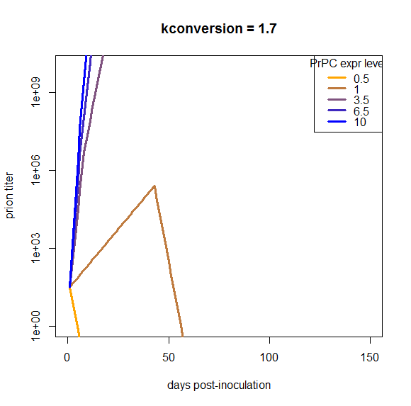
I phrase my interpretation this way because the above result came to me as a satisfying explanation to a problem I’d been having when trying to model the exponential growth of prions: there is no coefficient that gives reasonable results for a wide range of PrPC expression levels. I came to this conclusion after plugging in a bunch of different values and finding that nothing works. Here are a few examples, varying kconversion:
par(mfrow=c(2,2))  # make a 4-panel plot
for (kconv in c(.10,.30,.60,1.0)) { # try diff values of kconv in days^-1
    PrPSc0 = 10^1.5 # initial titer
    kdeg = log(2) / 1.5 # degradation constant in days^-1
    #kconv = .50
    times = 0:150 # model 0 dpi to 300 dpi
    prpsct = function(prpc,t) { # function implementing the model discussed here
      return ( PrPSc0*exp((prpc*kconv-kdeg)*t) )
    }
    plot(NA,NA,xlim=range(times),ylim=c(1,10^10),log="y", # empty plot over 300 days and 10 log10s
         xlab='days post-inoculation', ylab='prion titer', main=paste("kconversion = ",kconv,sep=''))
    colorvals = data.frame(prpc=c(.5,1,3.5,6.5,10),k=colorRampPalette(c("orange","blue"))(n=5),
        stringsAsFactors=FALSE) # this is necessary to have R read the hex colors as strings
    for (prpc in c(.5,1,3.5,6.5,10)) {
        points(times,prpsct(prpc,times),type='l',lwd=3,col=colorvals$k[colorvals$prpc==prpc]) # fill in the curves for each PrPC expr level
    }
    abline(h=PrPSc0)
    legend('topright',legend=colorvals$prpc,col=colorvals$k,lwd=3,pch=NA,title="PrPC expr level",bg='white') # add a legend for curve colors
}
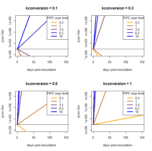
At low values of kconversion where the high overexpressers reach a titer of 109 ID50 in tens of days, the wild-type and even moderate overexpressers can’t support prion replication at all and simply degrade everything. Once kconversion gets high enough to give a reasonable slope for the het knockouts, the overexpressers are reaching terminal prion titers almost instantly.
how can we fix it?
All this shows that this model is wrong. What options do we have for fixing it? Here’s the model again for reference:
Or rephrased in “plain” language:
 = PrP^{Sc}_0 e^{(k_{conversion}PrP^{C} - k_{degradation})t}")
I’ll start by arguing there are some basic things about the model that we can’t just throw out. We cannot just remove [PrPC] from the first term since there is clearly a genotypic difference based on PrPC expression level. We also cannot remove [PrPSc] from the first term (throwing out the exponential growth assumption) because it is hard to see how you would gain 7 or 8 log10 ID50 in tens of days without exponential growth, and moreover the infectivity titer growth data from Sandberg 2011 Fig 1b look roughly linear in the log space, implying that growth is indeed exponential.
One possible improvement is to acknowledge that each mouse model must have a different value of initial PrPSc a.k.a. T0. We could model the way that excess PrPSc is degraded in the first few days after inoculation, and we’d find that the mice with higher PrPC expression are able to “save” more of the inoculated dose of infectivity, so they’d start with a higher T0 by day 4. That wouldn’t help our model – in fact, it would make it even yet harder to reconcile the difference in growth rates between high- and low-expressing mice.
Another point is that I assumed that PrPC expression is constant over the disease course, i.e. that S(t) = S0 for all t. We could consider changing this assumption to account for the PrPC downregulation that is reported to occur about halfway through the incubation period. But if you look at the plots above, our curves are off by so much that just dropping the growth rate by a factor of 2 for half of the time is not going to make up the difference, and applying it uniformly to all of the genotypes isn’t going to bring them closer together. I confirmed this in a simulation:
At this particular value of kconversion, wild-type mice replicate prions until the downregulation occurs, and then once it occurs, they completely clear the infection. That’s not what really happens in vivo, and moreover, this downregulation does nothing about the problem that the overexpressing mice are able to continue replicating with barely an inflection in the curve right through the downregulation, and the het knockouts can’t support replication at all. So, holding everything else about this model as is, downregulation does not remotely begin to make the model look plausible.
Let’s get down to some fundamentals. What about my assumption equating PrPSc with infectivity? That’s surely wrong – why, just look at the fact that PrPSc continues to rise during the neurotoxic end game (see evidence cited in point #2 of Facts about prion kinetics). Furthermore, this was the assumption that Ghaemmaghami 2007 had to throw out in order to get his model of kinetics in cell culture to make sense. So it seems like an obvious target.
If we go that route, one change to make would be to say that the more PrPSc there is, the smaller a fraction of it is infectious – in fact, you can’t get above 109 ID50s no matter how much PrPSc you have. We could give various biological explanations for this – Ghaemmaghami 2007 offers the sequestration of excess PrPSc into benign aggregates or the saturation of lipid rafts or co-factors needed for conversion. Since infectivity appears saturable, one option that occurs to me would be to borrow a model from another saturable system – Michaelis-Menten enzyme kinetics. Borrowing a page from that book, we could set an infectivitymax value and decree a Km value (the value of PrPSc at which infectivity is ½infectivitymax) and then:

The equations would then have to be re-written and re-solved to allow infectivity and PrPSc to have distinct values. I’m not sure whether this option will prove interesting or not and I may explore it in a future post.
Another possibility to consider is that kdegradation might not be constant. PrPSc has been shown to interfere with the proteasome [Kristiansen 2007] and vacuolation in prion disease might be taken to suggest problems with lysosomes too
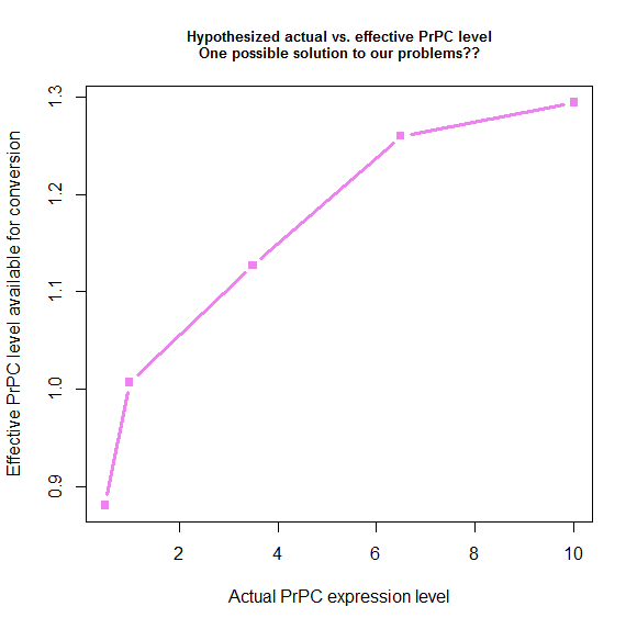
Yet another option we could consider would be a saturable model for PrPC. Biologically, this would mean that, say, 10-fold overexpression only results in, say, 1.8x as much PrPC being available for conversion, because the rest can’t find a spot in lipid rafts or something. This strikes me as being the most trivially easy way to correct the problems of the model that I’ve highlighted in this post. In fact, we can pretty easily figure out what the saturation curve would have to look like. Remember that I rearranged the equation to:
If we plug in some plausible values like ln(Tonset/T0) ≈ 17 and kdegradation = ln(2)/1.5d = .46d-1, then we can find a reasonable value for kconversion based on wild-type mice:

This gives kconversion ≈ .59. If we then plug this in along with tonset for the other genotypes, we can solve for what I’ll call Seffective on the left side.

Plotting what this spits out gives us a nice-looking saturation curve:
s_eff = function(tonset) { # calculate "effective" PrPC level
   return ( 28.8 / tonset + .78 )
}
explevel = c(.5,1,3.5,6.5,10) # PrPC expression level
symptoms = c(290,131,87,64,60) # time to symptoms
plot(explevel, s_eff(symptoms - 4), type='b', pch=15, lwd=3, col='violet',
    xlab = 'Actual PrPC expression level', ylab = 'Effective PrPC level available for conversion',
    main = 'Hypothesized actual vs. effective PrPC level\nOne possible solution to our problems??',cex.main=.8)
We derived these values by plugging things into the model, so by definition, if we use these values, the model has to fit the data. Here’s what that ends up looking like:
times = 1:300
kconv = .59
kdeg = .46
PrPSc0 = 10^1.5
prpsct = function(prpc,t) { # function implementing the model discussed here
  return ( PrPSc0*exp((prpc*kconv-kdeg)*t) )
}
effective_prpc = s_eff(symptoms - 4)
plot(NA,NA,xlim=range(times),ylim=c(1,10^10),log="y", # empty plot over 300 days and 10 log10s
     xlab='days post-inoculation', ylab='prion titer', main='Model "fixed" by PrPC saturation assumption')
colorvals = data.frame(effective_prpc=effective_prpc,prpc=c(.5,1,3.5,6.5,10),k=colorRampPalette(c("orange","blue"))(n=5),
    stringsAsFactors=FALSE) # this is necessary to have R read the hex colors as strings
for (prpc in effective_prpc) {
    points(times,prpsct(prpc,times),type='l',lwd=3,col=colorvals$k[colorvals$effective_prpc==prpc]) # fill in the curves for each PrPC expr level
}
abline(h=PrPSc0)
abline(h=10**9)
legend('bottomright',legend=colorvals$prpc,col=colorvals$k,lwd=3,pch=NA,title="PrPC expr level",bg='white') # add a legend for curve colors
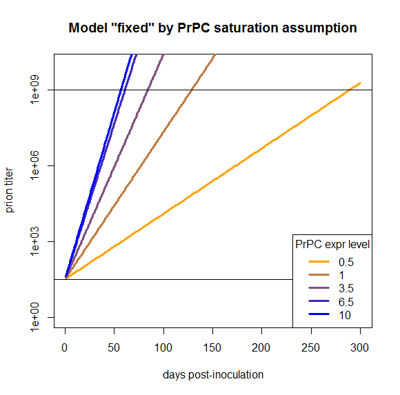
The fact that this model now works is a tautology and so, arguably, not that interesting. But my purpose in doing all this modeling was to see what we would need to change in order to have a model that does work, and here we’ve found one thing we can change in order to make it work. That’s distinct from, say, modeling PrPC downregulation or differing T0 values, which I’ve argued here would not fix this model.
To see whether the PrPC saturation idea is indeed a good way to explain the observed data, I’ll plan to look at more different types of data. So far I’ve only thrown one dataset against the “exponential model” hypothesis. Another thing I’ll want to consider in a later post is the relationship between inoculated dose and incubation time as documented in [Prusiner 1982b]. Depending on how the model fits that data, it could also be extended to overexpressing mice using data from Fischer 1996 (ft).
A final note: it is interesting to speculate on why the half-life of infectivity upon inoculation seems to be so much faster than the half-life of PrPSc. One possibility is that the smaller multimers of PrPSc, which may be more infectious [Silveira 2005], are easier to degrade than larger aggregates. Another appealing possibility would be that extracellular PrPSc is easier to degrade than intracellular or membrane-anchored PrPSc. For instance, maybe macrophages or astrocytes can chew up extracellular PrPSc more rapidly than neurons can degrade their own PrPSc.
All in all: not yet clear this model has done anything useful, but it has at least provided a starting point for discussing what sorts of biological phenomena could or could not explain the observed kinetics of prion infection.

About Eric Vallabh Minikel
Eric Vallabh Minikel is on a lifelong quest to prevent prion disease. He is a scientist based at the Broad Institute of MIT and Harvard.