Genetics 24: 'Complex traits, heritability, and the genetics of populations'
These are my notes from lecture 24 of Harvard’s Genetics 201 course, delivered by Steve McCarroll on November 19, 2014.
Why perform exome sequencing?
This part of the lecture is a continuation of the last lecture on monogenic disorders.
Whole genomes vs. whole exomes
Whole exome sequencing remains a preferred alternative to whole genome sequencing in most cases. It is still a few times cheaper (perhaps 1/5 the cost), and it produces less data (a good exome is 15GB, a good whole genome is 200GB) which makes it computationally easier to manage, while it still includes the parts of the genome that we have the best ability to interpret functionally. For further comparison of whole genome and whole exome, see this post.
Exomes vs. linkage mapping
Certain kinds of genetic causality cannot be uncovered with linkage analysis, but can be uncovered with sequencing. For example, de novo mutations, which are a plausible inheritance model for rare, sporadic congenital disorders with low sibling recurrence. See for instance Ben Neale and Mark Daly’s landmark paper on de novo mutations in autism [Neale 2012].
One of the first, if not the first, genetic disorder to be solved using exome sequencing was Kabuki syndrome, which turns out to be due to heterozygous loss-of-function mutations in the haploinsufficient gene MLL2 [Ng 2010]. The researchers sequenced the exomes of 10 trios, and applied aggressive filtering, removing variants that were seen in public databases such as dbSNP and 1000 Genomes, and looking specifically for loss-of-function mutations. They also used the clever strategy of ranking the patients according to how closely their phenotype resembled canonical features of Kabuki syndrome, as outlined in Table 2. Through these strategies they were able to find that 9 of the 10 patients had rare variants in MLL2, four of which were clear loss-of-function variants.
Polygenic inheritance
The study of polygenic traits and disorders in humans has been informed in large part by agricultural genetics. Some of this is reviewed in [Visscher 2008].
Consider the example of Angus cattle, which were imported from Scotland in the 1900s and have been selectively bred to increase meat yield. In each generation, bulls from the right tail of the distribution of meat yield are selected to contribute sperm for the next generation. This progressively shifts the mean meat yield upward in each generation. As a result, meat yields have increased linearly ever since the 1950s. This was somewhat surprising. Initially, people thought that meat yield would plateau after several generations once all of the favorable alleles had become fixed. And if meat yield were a mono- or oligogenic trait, that might indeed be expected. Instead, the heritability of meat yield has remained high even as average meat yield has increased, which is consistent with polygenic inheritance.
Francis Galton was Charles Darwin’s half-cousin and a contemporary of Mendel. Whereas Mendel studied binary traits, which turned out to be monogenic (or “Mendelian” as we now say), Galton studied quantitative traits, which he called “blending characters” and which we now recognize as being polygenic. Galton posited that quantitative traits owed to “multifactorial” inheritance.
Distinguishing which human traits are mono- or polygenic is not trivial. Traits with continuous variation, such as height, are clearly polygenic, but the converse is not true, meaning that binary traits are not necessarily monogenic. For instance, whether you get (late-onset) Alzheimer’s disease is a binary trait, yet many genes contribute to risk [Hollingworth 2011]. How, then, can one determine whether a trait is polygenic? Polygenic traits will tend to aggregate in families but not to show Mendelian segregation.
Heritability of polygenic traits
I’ve reviewed some of the approaches for measuring heritability in this post.
Parent-offspring regression
Galton invented the idea of parent-offspring regression for quantitative traits. In this technique, you regress the “mid-parent value” (average of the two parents’ traits) against the child’s value, and the slope of the regression line is taken to be an estimate of additive heritability (h2). If you only have the trait available for one parent, you can perform single parent-offspring regression, in which case twice the slope of the regression line is an estimator of additive heritability. In human populations, however, parents and children tend to share more of their environment than two random people plucked off the street. Therefore, the correlation between their phenotypes should be considered as an estimator of additive heritability plus environmental contributions, or in other words, an upper bound on heritability. (Self promotion on: I’ve found that parent-offspring regression is also vulnerable to ascertainment bias for some phenotypes [Minikel 2014]).
Twin studies
Twin studies were invented to control for this environmental confounding. Any set of twins is assumed to share about the same amount of environmental influence, but monozygotic (MZ) twins share 100% of their genome, while dizygotic (DZ) twins share just 50%. Therefore, Falconer’s formula considers additive heritability to be twice the difference between correlation between MZ twins and correlation between DZ twins:
h2 = 2(rMZ - rDZ)
Intuitively, this makes sense because a trait that is no more shared between MZ twins than it is between DZ twins must just be environmental.
Modern approaches
Though not mentioned in lecture, I feel compelled to add a few modern techniques. Sibling IBD regression compares phenotypic similarity in siblings with different amounts of genome sharing, taking advantage of the fact that sib pair IBD is normally distributed ~50% ± 4% [Visscher 2006]. GCTA [Yang 2011] uses genome-wide SNP data to estimate heritability based on genetic similarity between unrelated individuals. LD score regression [Bulik-Sullivan 2014] is a brand new approach to discriminate true polygenicity from bias in genome-wide association studies.
Limitations and caveats regarding heritability
- Heritability is an abstract concept that in no way tells you which genes contribute.
- Heritability is a population-level concept with only limited predictive value for individuals.
- Measured heritability depends upon the variance in environment in the population being studied. For instance, heritability estimates for some traits are higher in populations in Europe than in individuals of European descent in the United States, which is believed to be because there is greater environmental variability in the U.S. For this reason, a heritability estimate is meaningful only within the context where it is measured. This also means that heritability estimates do not explain differences in the mean value of a trait between different populations.
- Heritability does not provide a bound on the potential effect of therapeutic interventions.
As an example, consider that the additive heritability of human height is estimated to be about 80%. Yet mean height has increased dramatically in the last 300 years, a time scale in which the genetic composition of the population has not changed appreciably, reflecting a huge environmental contribution. This discrepancy can be reconciled by observing that the heritability estimates were made based entirely on modern humans, a cross-section which does not capture those huge environmental changes.
Similarly, the prevalence of many disorders, such as type 2 diabetes or peanut allergies, has increased dramatically in incidence within our lifetimes. This indicates that environmental factors strongly influence these traits, yet we also know that strong genetic factors exist, and therapeutic interventions based on these genetic factors can have enormous effects.
Mapping the genetic basis of polygenic traits
Last time we discussed recombination in families, where there are only 1 or 2 recombination events per chromosome per generation. In contrast, in populations, there have been thousands of recombination events since the most recent common ancestor of any two unrelated individuals. These recombination events are concentrated in recombination hotspots, where the hotspots are sites where PRDM9 site-specific recombinase preferentially acts. Mark Daly and others recognized that a consequence of this is that the human genome can be dissected into haplotype blocks where there is little or no recombination within blocks, and limited haplotype diversity within blocks [International HapMap Consortium 2003]. Haplotype blocks are variable in size (2 - 200kb) due to variation in how far apart recombination hotspots are.
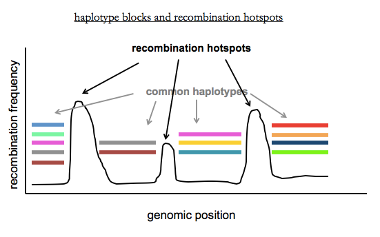
Within each block, there are a limited number of common haplotypes. Each block has on average 2-10 common haplotypes in African populations, and 2-5 in Europeans or East Asians (who have less diversity due to the out-of-Africa bottleneck). You can think of recent genetic variation as being sprinkled in on top of these common haplotypes. A consequence of the existence of haplotype blocks is that you don’t need to sequence every variant in a person’s genome in order to figure out what locus contains common variants that contribute to a phenotype. This last sentence foreshadows genome-wide association studies, the topic of Dr. McCarroll’s next lecture.

About Eric Vallabh Minikel
Eric Vallabh Minikel is on a lifelong quest to prevent prion disease. He is a scientist based at the Broad Institute of MIT and Harvard.