The quest for the structure of PrPSc
Three years into my quest to understand prions, I have remained too ignorant about structural biology. While I don’t expect to become a structural biologist myself, I decided I wanted to at least become literate in the subject - what is known, what is unknown, what are the methods, what are the challenges. So a few months ago, I wrote to Holger Wille to ask if he could recommend some reviews to get me acquainted with the subject. This led to my post last month about the structures of PrPC, and now with some more time spent reading, I’ve written this post about efforts to find the structure(s) of PrPSc.
I started by reading the three review articles Holger suggested [Surewicz & Apostol 2011, Diaz-Espinoza & Soto 2012, Requena & Wille 2014]. It immediately seemed to me that the story of the quest for a structure of PrPSc is a story of methods. For soluble, crystallizable proteins we’ve had X-ray crystallography and solution NMR for decades, techniques which have made it possible to get high-resolution structures. For insoluble, non-crystalline solids like PrPSc, we just don’t have a method in the toolkit today for completely solving them. Instead, to understand the state of the science of these structures is to understand the methods available, what they can and cannot achieve, and what pieces of information we have learned from each. I’ve therefore structured this post around the various methods used to obtain structural information about PrPSc.
As I’m new to this subject, my omissions and factual errors are sure to be both numerous and egregious. Corrections are very welcome.
Proteinase K digestion

Above: prion strains differ in whether residues 82-97 are accessible to proteinase K, so PK-digested samples result in different molecular weights. From [Schoch 2006], Figure 2.
Some of the earliest data indicating that prion strain properties were encoded in conformation came from limited digestion with proteinase K. If you digest PrPSc in high concentrations of PK at biological temperatures for a long time, PK will digest all of the protein and abolish infectivity. But under limiting conditions (say, 20 μg/mL for 1h at 37°C), PK will only digest the readily protease-accessible N terminus of PrP, which has a different extent in different strains of prions. You can then run the digested protein on a Western blot to figure out its size and what antibodies it will react with. In so-called type 1 strains, limited PK digestion leaves a 21 kDa fragment behind, while in so-called type 2 strains, a 19 kDa fragment remains. While the exact cut sites are variable, type 1 seems to correspond to cleavage at residue G82, and type 2 to cleavage at S97 (human numbering) [Parchi 2000]. This suggests that the segment from residues 82-97 is protected in some strains but exposed in others. The facts that (1) these properties can be transmitted faithfully to new PrP molecules in a cell-free reaction [Bessen 1995] and (2) these properties can be generated by genetic mutations (D178N and E200K) and then transmitted faithfully to mice expressing PrP without these mutations [Telling 1996] were two important pieces of evidence for the idea that protein conformation holds strain information. However, these observations are very low-resolution and we still don’t know much about the nature of the structural differences that give rise to differential protease accessibility of residues 82-97.
Besides the 21 and 19 kDa bands of canonical type 1 and type 2 strains, many other PK-resistant PrP fragments have been observed over time. For instance, many PRNP mutations with a GSS phenotype give rise to an 8 kDa protease-resistant fragment [Parchi 1998] and one prion strain generated de novo in PMCA has a 15 kDa fragment [Wang 2010]. Over ten different exact PK cleavage sites have been mapped in hamster 263K and drowsy (DY) prions [Sajnani 2008] and in anchorless prions [Vazquez-Fernandez 2012], which begins to give more detailed conformational information.
Antibody reactivity
The 3F4 epitope (KTNMKHM, residues 106-112 in human or hamster PrP) is accessible to the 3F4 antibody in natively folded PrPC and in GdnHCl-denatured PrP, but buried and inaccessible in PrPSc. Different prion strains require different amounts of GdnHCl to denature them enough to expose this epitope, which is the basis of the conformation-dependent immunoassay and was one additional piece of evidence that strain information is encoded in conformation [Safar 1998]. However, this doesn’t give very high resolution information about the structure of PrPSc.
There have also been efforts to use other antibodies to figure out which parts of PrP are buried or exposed in PrPSc. At Prion2014 Day 2 Surachai Supattapone said his lab is using this technique to probe the structural differences of infectious vs. “protein-only” PMCA-propagated PrPSc - still unpublished.
Fourier transform infrared spectroscopy (FTIR)

Above: drying protein onto the surface of a diamond for FTIR.
For FTIR, a pure preparation of the protein of interest is suspended in a small amount (say, 2 μL) of water. I say “suspended” rather than dissolved, because in many cases, such as PrPSc, the protein is insoluble. This suspension is then pipetted onto the flat surface of a synthetic diamond, which in the above photo appears as a tiny hole recessed in the middle of the steel disc. Next you want to dry the protein onto the surface of the diamond. You could do this by blowing air onto the surface, but then you’d be contaminating your protein with particulates, so instead you blow pure N2 across the surface until the protein is dry. Now you want to see how much light the protein absorbs at a variety of wavelengths. Different protein secondary structures have bonds which absorb light at different wavelengths. Which wavelengths are relevant? Well, by convention, people refer to wavenumber rather than wavelength in IR, and they use the unit cm-1. In those units, the range used in FTIR is 1500 to 1800 cm-1. To put this in perspective, 1800 cm-1 is a wavelength of (1/100)/1800 m ≈ 5.6 μm, and 1500 cm-1 is ~6.7 μm. Recall that the visible spectrum is about 400 to 700 nm - so for comparison, the IR spectra used in FTIR are about 5600 to 6700 nm, which is what people call the “mid-wavelength infrared”.
Now, you might think that an intuitive way to measure absorbance at all of these different wavelenghts would be to first shine a 5600 nm light at the sample, and measure how much is absorbed, then a 5601 nm light, then a 5602 nm light, and so on. In fact, FTIR manages to achieve essentially the same measurement - how much light is absorbed at each wavelength - in a different way: instead of emitting each wavelength separately, it emits a number of different mixtures of wavelengths, then uses a Fourier transform to back into how much light was being absorbed at each individual wavelength. While conceptually complicated, this is not computationally intensive, and the computer connected to the IR machine will display the absorbance at different wavelengths (or actually, by wavenumbers in cm-1) in real time as you run it.
How does one interpret absorbance in different infrared wavelengths to give information about protein structure? The go-to reference seems to be [Surewicz 1993]. As Surewicz notes, the interpretation is non-trivial. The classical view has been that α-helices absorb a lot of light in the 1650-1658 cm-1 range, while β-sheets absorb in the 1620 to 1640 cm-1 range. The intensity of these bands can even be construed to give quantitative information about the percentage of β-sheet and α-helical content. However, there are notable exceptions - proteins whose high-resolution structure has been solved by NMR or X-ray crystallography and contain no alpha helices or no beta sheets, yet which appear to have bands in the 1650-1658 or 1620-1640 range respectively.
Indeed, though we don’t have a high-resolution structure for PrPSc, it may be one such exception. The structure of PrPSc - in this case, hamster brain-derived 263K prion fibrils - was first probed by FTIR by [Caughey 1991]. Figure 5 from that paper shows the FTIR data interpreted in terms of turns, alpha helices and beta sheets:

The peak at 1657 cm-1 falls right with in the canonical α-helix range and is interpreted to mean that PrPSc has ~17% alpha helical content. The Prusiner group completed similar studies a couple of years later and similarly concluded that PrPSc contains 21% alpha helix [Pan 1993].
However, the consensus today is that PrPSc is in fact entirely devoid of alpha helices. Byron Caughey noted this in his talk at Prion2014, and a review by Jesus Requena and Holger Wille explains that the 1657 cm-1 band is now believed to correspond simply to turns between beta sheets [Requena & Wille 2014]. This shift in thinking occurred in part because other techniques such as hydrogen/deuterium exchange indicate the absence of any alpha helices [Smirnovas & Baron 2011]. It is also supported by studies of synthetic amyloid fibrils made of recombinant PrP - although the structure of these fibrils is also unsolved at any high resolution, they are believed to have a wholly beta sheet structure, and yet they, like PrPSc preparations, also contain a peak on FTIR corresponding to ~1657 cm-1 [Cobb 2007, Lu 2007, Smirnovas & Baron 2011].
Circular dichroism

Above: a machine for performing circular dichroism.
Circular dichroism means differential absorptions of left vs. right-handed polarized light. The CD machine emits left and then right-circularized light through a sample and measures how much of each is absorbed. The underlying principle is that polarized light interacts differently with molecules of different chirality. To understand this I had to think back to the story of how chirality was discovered by Louis Pasteur, looking at crystals of tartaric or paratartaric acid in wine - two small molecules with identical molecular formulas but opposite chirality, which polarize light differently. In the case of proteins, all of the individual amino acids are levorotary no matter what, but the protein can take on different chiralities depending on its secondary structure and conformation. The relevant range of wavelengths for CD analysis of proteins is the near ultraviolet, and specifically, alpha helices have negative bands at 222 and 208 nm and a positive band at 193 nm, while beta sheets give a negative band at 218 nm and a positive band at 195 nm [Greenfield 2006]. These signals are, however, confounded with the fact that aromatic amino acids (F, W and Y) themselves have differential absorbance at various wavelengths. Therefore it is customary to just plug your CD spectra into a program that deconvolutes the contribution of different signals.
Jiri Safar first applied this technique to PrPSc, either undigested or PK-digested to PrP 27-30, and with or without denaturing in various amounts of GdnHCl, to probe not only the structure of PrPSc but also its folding and unfolding [Safar 1993a]. The CD spectra for undigested PrPSc, for instance, are shown in Figure 2:

These data were interpreted to indiate that PrPSc was 34% beta sheet, 20% alpha helix, and 46% turns and disordered parts. However, as explained by [Requena & Wille 2014], this interpretation was later rejected because recombinant prion protein amyloids, which were shown by other experimental techniques to lack alpha helices, had apparently similar spectra [Ostapchenko 2010].
Hydrogen/deuterium exchange
In hydrogen/deuterium exchange (variously abbreviated H/D exchange or HX), you measure the rate at which hydrogen atoms in your protein are exchanged for deuterium in the surrounding solution. This tells you which hydrogens are exposed to solvent (as opposed to buried inside the folds of the protein), and to some extent their secondary structure (hydrogens in beta sheets exchange less readily than alpha helices). After taking your protein (made with mostly normal hydrogen) and putting it into a D2O solution for several days, there are a number of ways you can then go back and figure out which hydrogens underwent exchange [reviewed in Engen 2009]. Deuterium changes the NMR, FTIR and CD spectra of proteins, so any of those methods can be used in combination with HX, but perhaps the highest-resolution method is HX with mass spectrometry (HXMS). In HXMS, you let the protein sit in deuterated water, then trypsinize it and perform mass spec to see which peptides acquired deuterium. This approach was used by [Smirnovas & Baron 2011] and showed that, in mouse brain-derived 22L PrPSc, the entire stretch from residue ~81 to ~167 and possibly all the way to ~224 exhibited very little deuterium exchange, consistent with all of those residues belonging to beta sheets. At Prion2014 Day 2, Surachai Supattapone also mentioned that his group is using HX to characterize the structure of prions propagated in PMCA with the minimal cofactor phosphatidylethanolamine. That work is still unpublished.
Chemical modification and mass spectrometry or antibody binding
In this approach, you can use various small molecule agents to covalently modify exposed (but not buried) amino acids), then use mass spec to figure out which residues were modified. In this sense, it is somewhat analogous to HXMS (above) but with chemical changes, rather than deuterium exchange, providing the difference in mass (or charge) to be picked up on mass spec. In the reported studies using this appraoch, tetranitromethane has been used to modify tyrosines [Gong 2011], acetic anhydride to modify lysines [Gong 2011], and bis(sulfosuccinimidyl) suberate to cross-link exposed N-termini [Onisko 2005].
In addition to changing the mass of tryptic peptides in mass spec, chemical reactions also abolish antibody reactivity, and this property has been used to discriminate prion strains based on which epitopes are exposed (and therefore can be chemically modified) [Silva 2012].
Electron microscopy

Above: negative stain transmission electron microscopy image of amyloid fibrils formed from mutant recombinant PrP. From [Groveman & Kraus 2015], Figure 4F.
Electron microscopy comes in several forms, all of which share the principle of throwing electrons at a sample. Because electrons have smaller wavelengths, they can achieve much higher resolution than photons. One relevant form of EM is transmission electron microscopy with negative staining. In this procedure, electrons are shot upwards from underneath a sample, and a sensor above the sample detects the electrons that get through. Larger atoms are better at scattering electrons, so taking your biological sample (which consists mostly of small-ish atoms like C, N, O and H) and surrounding it with heavier atoms (such as tungsten or uranium) is one way to get contrast between the biological material (which transmits most electrons) and the “negative stain” (which blocks most electrons from getting straight through).
The first hints as to the ultrastructure of PrPSc fibrils came from electron microscopy [Merz 1981, Prusiner 1983]. Prusiner purified PrPSc using the protocol described here and, using EM, found that prion fibrils had a diameter of ~25 nm and a length of 100 to 200 nm. Like the fibrils that by that point had already been seen in Alzheimer’s brains, these fibrils were “birefringent” and would stain with Congo red, thus meeting the functional definition of amyloid. Also, the fibrils were disordered and somewhat heterogeneous, unlike crystallized viruses, which are highly ordered.
That heterogeneity is part of what makes it difficult to get high resolution information out of EM. Recently, some investigators have started focusing on so-called anchorless or ΔGPI prions, as these are still infectious yet lack the GPI anchor and are unglycosylated, thus consisting of a more uniform pure protein. At Prion2014 Day 3, Jesus Requena described his and Holger Wille’s efforts to get structural information by averaging the dimensions and periodicity of negative staining in hundreds of transmission electron microscopy images from anchorless prions. That work is still unpublished.
When you perform transmission electron microscopy on 2D crystals of a protein, that’s called electron crystallography. Although PrPSc does not form 3D crystals that would be amenable to X-ray crystallography, it was observed that when you purify PrP 27-30 you sometimes get 2D hexagonal crystals in addition to amyloid rods [Wille 2002, see esp. Figure 1]. Given that these are clearly a different ultrastructure than the rods, and that both occur together, it’s not clear to me how we know that these crystals are actually infectious and not just a non-infectious off-pathway aggregate. But in any case, the advantage of 2D crystals is that, although EM still doesn’t have the power to resolve individual atoms, the structure is regular and so through image processing and Fourier transforms you can derive higher-resolution structural information. This approach has given some of the highest resolution (~7Å) information on PrPSc available right now [Wille 2002, Wille 2007]. By comparing PrP 27-30 to the 106-residue “miniprions” [Supattapone 1999] it was possible to get an idea of where residues 141-176 (which miniprions lack) and the glycan chains are located.
X-ray fiber diffraction and small angle X ray scattering
For proteins that are able to form 3D crystals, the highest-resolution structural information can often be obtained through X-ray crystallography, in which the diffraction of X-rays in the crystal is used to infer where each atom is. For proteins that don’t form 3D crystals, such as PrPSc, this isn’t possible, but because PrPSc does form fibrils, one can still get some information from X-ray fiber diffraction. In this technique, the fibril rod is modeled as being a cylinder, with the axis along the height of the cylinder being called the meridian and the axis through the cross-sectional diameter of the cylinder being called the equator. By rotating your sample and seeing how X-rays diffract from different sides of the fiber, you can get a 2D image like Figure 1 from [Wille 2009]. This technique performed on hamster brain-derived Sc237 PrP 27-30 and mouse brain-derived RML 27-30 precipitated with phosphotungstic acid, and one of the main conclusions seems to be that both structures contain a 19.2Å repeating unit, consistent with four rungs of β-strands each 4.8Å in height. This has been one constraint on structural models of PrPSc.
A related technique is to throw X-rays at the sample from a narrow range of angles and see how the scattering pattern changes; this is called small angle X-ray scattering and, similar to EM, has given information on the dimensions of prion fibrils [Amenitsch 2013].
Nuclear magnetic resonance (NMR)

Above: NMR device and spectra from Rob Tycko’s website.
I still don’t really understand how NMR works, except to say that you place the sample in a strong magnetic field to align all of a given atom (for instance, all of the hydrogens) with or against the field, and then you can get very high-resolution information about the structure of the molecule beacuse each atom will behave differently depending on what other atoms it is bonded to. Over 20 years ago, Kurt Wuthrich pioneered the idea of using solution NMR to find the structures of biomolecules, and this enabled the first structure of PrPC [Riek 1996]. But as the name implies, solution NMR requires that the biomolecule of interest be in solution, and PrPSc is insoluble.
A more recent approach is solid state NMR, which doesn’t require the protein to be soluble. Indeed, the only prion whose structure has been solved at high resolution, the HET-s prion of Podospora anserina, was solved by solid state NMR [Wasmer 2008], which seems to be a good sign that maybe other prions and amyloids could prove amenable to this approach too. Many such efforts are reviewed in [Tycko 2011].

Above: the solid state NMR structure [PDB# 2RNM] of HET-s amyloid, the only prion whose structure has been solved at high resolution. PyMOL code to generate this graphic: fetch 2rnm; bg_color white; hide everything; show cartoon; spectrum;
As for PrP in particular, several efforts have been reported. Solid state NMR has been applied to amyloids made of trunacated recombinant PrP corresponding to PrP 106-126 [Walsh 2009], PrP 127-147 [Lin 2010], and HuPrP 23-144 [Helmus 2008, Helmus 2010, Jones 2011], but only ~30 residues of HuPrP 23-144 are immobilized enough to resolve well on NMR. Full-length recombinant PrP has been studied as well - amyloid fibrils of SHaPrP 23-231 formed under denaturing and shaking conditions [Tycko 2010] or in 263K-seeded RT-QuIC [Groveman 2014]. These efforts have yielded various constraints on the set of possible models for the structure of these amyloids, though no one has yet obtained a high-resolution structure like that of HET-s. The recombinant amyloids being studied in ssNMR are generally not infectious, and it is not yet clear how their structures must relate to those of infectious PrPSc. For instance, both reported studies of SHaPrP23-231 fibrils [Tycko 2010, Groveman 2014] have been consistent with parallel in-register beta sheet (PIRIBS) conformations, a structure that apparently conflicts with some of the measurements obtained from brain-derived PrPSc.
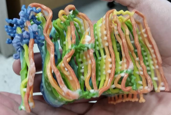
Above: Brad Groveman with a 3D printout of a theoretical PIRIBS model of RT-QuIC fibrils, proposed on the basis of solid state NMR data [Groveman 2014].
There must be some reason why solid state NMR cannot be applied to brain-derived PrPSc, or else someone would have done it, but I couldn’t find an explanation in any of the reviews I read.
Thoughts and conclusions
Given the challenges inherent in studying the structure of prions and amyloids, I reason that it must be the case that the structural biolgoists who choose to devote their careers to PrP are particularly ambitious individuals. If so, then I further speculate that they must each dream of one day writing up their manuscript entitled, “2.5Å structure of an infectious mammalian prion”. Is this indeed what the future holds, or is a gradual whittling-away at the structure with various low-resolution techniques the more likely road forward? After learning about the above techniques and results, I am left pondering two major questions:
- Is there any currently imaginable route to obtaining a high-resolution structure of PrPSc?
- If so, then once a structure is obtained, how will one be sure that the structure you’ve solved is indeed the same thing that is infectious?
I welcome any comments.

About Eric Vallabh Minikel
Eric Vallabh Minikel is on a lifelong quest to prevent prion disease. He is a scientist based at the Broad Institute of MIT and Harvard.