Differential scanning calorimetry

In the past couple of weeks, Sonia and I have learned how to perform differential scanning calorimetry (DSC). Here’s what we’ve learned.
What and why
DSC is a highly precise way of determining the melting temperature (Tm) of a purified protein. This technique determines melting point by comparing two solutions that are identical in terms of buffer conditions and differ only in whether a protein is present — hence “differential”. The solutions are heated in tandem in a scan from some starting temperature (say, 20°C) to some ending temperature (say, 110°C) — hence “scanning”. In the empty buffer solution, across the whole scan, as you put heat in, the temperature rises predictably. In the protein solution, it’s not so simple. In the beginning and in the end of your scan, the input of heat will raise the temperature of the protein solution predictably. But somewhere in between, there will be a range of temperatures where it takes a larger-than-expected amount of heat to raise the temperature by each 1°. That’s because the heat is going into unfolding the protein instead of going into raising the temperature. By comparing the curve of calories of heat added vs. temperature reached for your protein vs. your empty buffer, DSC can determine the melting point of your protein — hence “calorimetry”. To be precise in terminology, what DSC is measuring is heat capacity, the amount of heat energy needed to raise the temperature each degree, in units of kcal/°C. The output, Tm, depending on who you ask, may stand for either melting temperature or transition midpoint; in either case, it is the temperature at which heat capacity is maximized, which is also the temperature where 50% of the protein is unfolded.
DSC is useful because measuring the melting point of your protein allows you to identify conditions that cause the melting point to shift. For instance, if you add a small molecule ligand, it might thermally stabilize the protein, resulting in a higher Tm. Conversely, a change in buffer conditions, such as addition of denaturant or a less favorable pH, might result in a lower Tm. In some proteins, a pathogenic amino acid substitution may also reduce the Tm.
DSC is often used as a way to test small molecules’ ability to bind — and thermally stabilize — a protein of interest, usually as a secondary screen to validate hits from some larger screen. Two popular alternatives for secondary/validation screens are isothermal titration calorimetry (ITC) and surface plasmon resonance (SPR). Here are some considerations for deciding which assay is right for you.
- What makes DSC unique is its specificity for the subset of small molecule ligands that do thermally stabilize a protein, whereas the other techniques will only tell you whether a small molecule binds, not whether it stabilizes.
- DSC is very easy to get started with, requiring almost no assay development work, but is relatively consumptive of protein (200 μg per well). ITC requires similar amounts of protein, but SPR requires only tens of μg of protein. The devil’s bargain of SPR, then, is that you need to figure out a way to A) tether your protein to a surface, and B) still be convinced that it is folded correctly. This can be a significant undertaking.
- DSC is relatively slow, requiring over an hour per condition tested.
- DSC can miss weak binders (Kd > 500 μM)
- DSC is sometimes used in dose-response to determine Kd, but this only works if the binding is mostly entropically driven. SPR or ITC are preferred for Kd determination.
- One caveat to be aware of in DSC is that many proteins have a Tm that is dependent upon pH. Consider that if a compound is being tested at a particularly high concentration such as 2 mM, and comes as a dihydrochloride salt, its release of protons can overwhelm a 10 mM phosphate buffer and change the pH enough to alter the protein’s Tm, possibly resulting in a false positive or a false negative. If need be, this can be overcome by using a stronger buffer. Note that compounds that are not HCl salts are usually not problematic.
How
The Broad uses the GE MicroCal VP-Capillary DSC. Here’s a diagram of my limited understanding of the device:

The test samples are loaded into these deep well 96-well plates and then reusable plastic mats are pressed on to cover them. (After use, the mats are simply rinsed 20-30 times in de-ionized water).

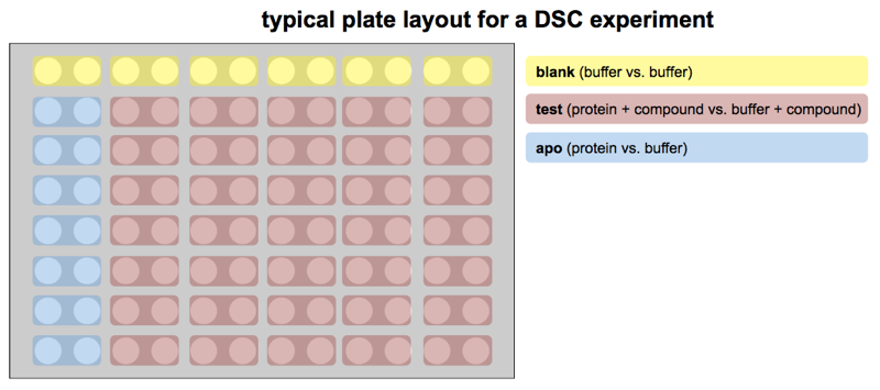
The layout is as follows. First, every protein sample must be in an even-numbered column, with the corresponding no-protein reference buffer in the odd-numbered column to its left. The machine is hard-coded to compare adjacent cells in this way; no other arrangement is allowed. Although the machine can run wash cycles between each pair of wells, and supposedly starts at the same temperature for each run, it is still considered best practice to run several blank samples (pairs where both sample and reference are no-protein buffer) across all of row A before running any actual protein, in part to reset the “thermal history” of the machine.
In a typical experiment, one might be comparing protein by itself (the “apo” state) to protein with any of several different candidate small molecule ligands. Remember that this comparison means you are measuring protein, with just buffer as a reference cell, to get a Tm for the “apo” protein, and then also measuring protein + ligand, with buffer + ligand as a reference cell, to get a Tm for the protein in the presence of a ligand. Thus, comparing two conditions requires four cells — remember that each and every protein sample must have an identical-except-for-protein reference cell next to it.
In practice, if you are testing a battery of compounds, you will want a series of “apo” controls, which by convention are placed in column 2 of every row (with column 1 as its reference). Having more than one copy of the “apo” has two benefits. First, you get a distribution of Tm measurements for your protein. That way, when you need to decide which compounds you deem to have thermally stabilized the protein, you can ask, for instance, which ones gave a Tm that would have had a Z score of at least 3 compared to the “apo” distribution. Most proteins will, in their “apo” state, have Tm values within ±0.1°C or 0.2°C, while a ligand will often raise Tm by 1°C. Second, many proteins are unstable over time, particularly in the presence of DMSO, and one DSC plate takes a couple of days to run. Remember that if your compounds are in DMSO stock solutions, then your protein + compound sample will be some percent DMSO, and so your “apo” sample should be that same percent DMSO in order to be a good control. Placing “apo” samples all down column 2 ensures that if your protein’s melting point is dropping over the course of a couple of days in 2% or 4% DMSO, at least you’ll know it and be able to control for it.
With all that said, here is a diagram of the typical experimental layout:
Another point of note related to layout is that the DSC software does not allow you to add in a “wait” step in your experiment. So if you need time to pass between one reading and another reading — for instance to check the stability of your protein over time — then your only option is to add in a bunch of blank (buffer vs. buffer) samples in between to kill time.
The machine takes up about 375 μL of each sample and of its corresponding buffer; to be safe, one should add 400 μL to each well. This little bit of excess ensures the machine won’t run dry, and also means that you’ll have a bit left over at the end. This can be useful: for instance, sometimes one compound will look like it has a potential covalent liability. If it gave a particularly large thermal shift in DSC, then afterwards, you might want to throw the sample on the mass spec to see whether the compound had indeed covalently attached itself to your protein. The protein sample should be at 0.5 mg/mL, which means you’ll use 200 μg of protein for each condition. Note that since the calorimetry here is “differential”, it is of paramount importance that the buffer in the no-protein reference be perfectly matched. And you’ll need a fair amount of that buffer, so be sure to save enough after dialyzing your protein.
The machine will heat the samples from some starting temperature to some finishing temperature. While the plate is sitting in the drawer it is stored at 7°C, and by default the scan starts at 15°C, but if you know your melting point is well above room temperature, you can just start the scan at 20 or 25°C to save some time.
Our experience with PrP
To get more into the details of how to run DSC, I’ll share exactly what we did. We would like to use DSC to study PrP, so as a first step, we ran a pilot experiment just to check the baseline melting temperature and stability in DMSO and over time. We used this batch of recombinant HuPrP23-230, dialyzed into 20 mM HEPES at pH 6.8. We concentrated it to 0.94 mg/mL, then diluted it back down to 0.5 mg/mL (the desired concentration for DSC) in the dialysis buffer in the process of setting up the plate.
Note that normally, one would be comparing the Tm of protein + DMSO + compound against just protein + DMSO, so the protein + DMSO condition would be considered “apo”. But since our goal was to first check what concentration of DMSO was tolerated, we considered the protein without DMSO as “apo” and the DMSO as the “compound”.
Here’s how we set up our plate:
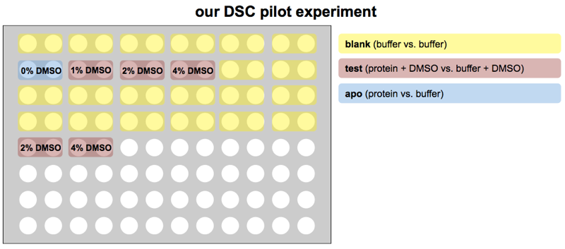
The blank samples at the end of row B and all of rows C and D are just to stall for time. Each pair of wells takes 80 minutes, so this layout means about 23 hours will pass between the “apo” and the 2% and 4% DMSO in row E, enough to get some idea of whether sitting in DMSO for a day lowers PrP’s melting point.
After loading these samples into the deepwell plate, we pressed one of the reusable plastic mats onto the top of the plate. We then placed the plate into a position in one of the drawers on the left side of the machine, and queued up our run in the Origin software’s Controller screen. We had some idea both from the literature [Calzolai & Zahn 2003, Nicoll 2010] and from doing our own circular dichroism melting curve that the melting point of our protein, HuPrP23-230, would be plenty high, somewhere in the 65-75°C range, so we set the boot temperature to 20 °C (still plenty conservative) rather than 15°C (the default). We used a screen rate of 120°C/hour, so in principle, each scan from 20°C to 110°C should only take 45 minutes. It’s the various washing and loading steps that make each scan end up taking a total of 80 minutes.
Here are a few more steps to set up the run in the control software:
- Select the plate position within the drawer and drag to select the wells in use, which generates a table of sample wells.
- In that table, highlight all and click “clean before next sample” to insert wash steps between reads (apparently this is not the default). The word “yes” will now appear in the “clean” column for every sample.
- Set the sample type for each well: BB (buffer-buffer), STD (“apo”), or CPD (test compound, or in our case, DMSO). Also give each sample a unique name, even if it’s just bb1, bb2, etc. Note that this part of setting up the experiment is super tedious. Your time-saving alternative is to create an Excel file describing the experiment and then just load that into the software.
- Set a path for saving the data. This folder will get one
.dscfile per scan written into it, along with a metadata fileexpt1.pl2describing the experiment. Of note, that metadata file does not contain the time at which each sample was run. The only way I’ve been able to figure out how to get that is from the operating system (last modified date of each.dscfile).
A final thing to do before clicking “Start” is to confirm that pressure is at about 70 psi, and that the carboy is at least half full of milliQ water and that there is sufficient water and Contrad-70 in the wash flasks.
Results
Agreeably, the software writes out the raw data in plain-text .dsc files (here’s one example, from our “apo” protein scan), albeit without column names, and without any definition of the large amount of metadata in the header. I couldn’t find a spec for these files online, so I just browsed the data in the provided software, which actually works reasonably well. The key result one is interested in is the marginal amount of heat that must be added in order to achieve each additional fraction of a degree of temperature increase, in protein compared to buffer, as a function of temperature. This amounts to a curve with an x axis in °C and a y axis in cal/°C. To wit:
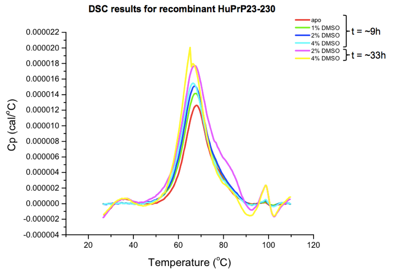
You can also export a summary table as a CSV, which will just have the melting point called for each sample. As you can see from the curves above, there is actually some melting going on over a range of tens of degrees. The Tm is simply considered to be the peak of that curve, which is the point at which 50% of the protein is melted. (There are also metrics for quantifying the width of the curve, for instance, the width at the half-maximal height.)
Here are the summary stats for our samples:
| condition | time (h) | Tm (°C) |
|---|---|---|
| 0% DMSO (“apo”) | 9 | 67.88 |
| 1% DMSO | 11 | 67.74 |
| 2% DMSO | 12 | 67.09 |
| 4% DMSO | 13 | 66.44 |
| 2% DMSO | 33 | 67.27 |
| 4% DMSO | 35 | 65.17 |
The conditions tested had the expected direction of effect: DMSO dose-dependently and time-dependently destabilizes PrP. For instance, the 4% DMSO sample that was run only a few hours after the “apo” sample came in about 1.5°C lower than “apo”, and the 4% DMSO sample run another 24 hours later weighed in another 1.3°C lower. Now, none of these differences are enough to preclude testing compounds at a 4% DMSO concentration — 65°C is still a perfectly respectable melting temperature — but it does illustrate the need for proper controls. This is why you need multiple “apo” scans at the same DMSO concentration, across the time course of the experiment, so that you’re comparing apples to apples, and you can control for the effects of time. Since this was just a small pilot experiment, we also don’t know how much of this is just stochastic variability between scans, so having multiple “apo” scans is important for that reason too.

About Eric Vallabh Minikel
Eric Vallabh Minikel is on a lifelong quest to prevent prion disease. He is a scientist based at the Broad Institute of MIT and Harvard.