Color transformations for segmenting complex images
Over the past several weeks I’ve spent a lot of time playing with both convolutional networks and CellProfiler, trying to find a good way to segment the mouse brain images. It’s not easy. CellProfiler does really great with immunostaining where you’ve got bright fluorescent cells, uniformly sized and shaped, against a black background. In fact, even without changing any of the default settings you can get a pretty bomb segmentation going:
(Left: uniform immortalized cells with three stains, the blue of which is DAPI staining the nuclei; Center: just the blue color channel; Right: an almost perfect segmentation by CellProfiler without changing a setting)
Not so much for light microscopy (i.e. measuring reflection, not emission) from multi-stained in vivo sections with a lot of different cell types. Watch while CellProfiler totally strikes out on segmenting this H&E mouse brain image (scale bar 100 um):
(left: original; center: grayscale by averaging & inverting RGB; right: CellProfiler’s segmentation with all default settings)
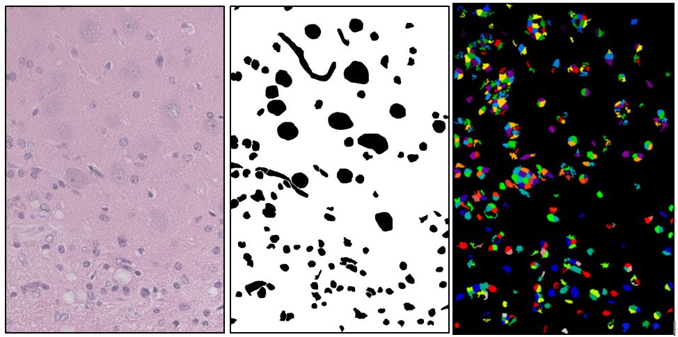
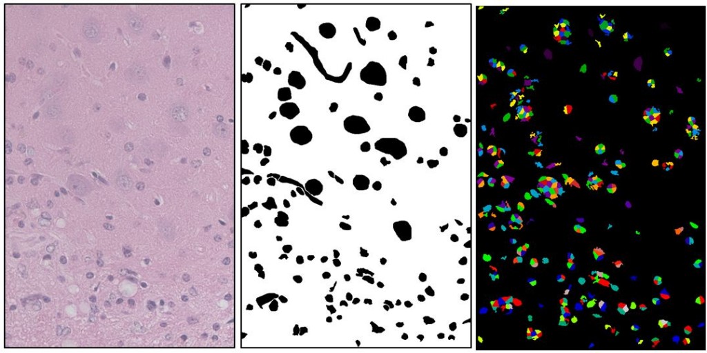
I figured CellProfiler surely can do better than this– it is a rather large software package with a LOT of different segmentation settings, it’s just that the typical biologist (or even bioinformatician) using it doesn’t know the difference between the Otsu Global and MoG Adaptive thresholding methods and won’t know how to pick the settings that will work for their images. So I spent much of the last few weeks implementing a machine learning approach in Python that cycles through the different CellProfiler settings to see which performs best against a provided ground truth. With this I was eventually able to do a bit better, but still not well enough for any real analysis:
(left: Source image, center: Manually drawn ground truth showing astrocyte nuclei (small), neuron nuclei (big), and blood vessels (squiggly). right: Best segmentation found after 400 iterations of a genetic algorithm on CellProfiler settings. This segmentation has a Rand index of .86. It found many of the desired objects but a lot of extra stuff as well).
So far I haven’t been able to do a whole lot better with my convolutional network implementation in Python either. This I think is largely because I still haven’t quite worked out all the bugs in my implementation:
(left: Small source image used for testing; mid-left: Grayscale (averaged) inverted version; mid-right: Ground truth; right: Output of convolutional network)
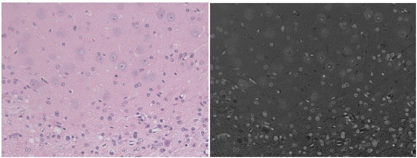
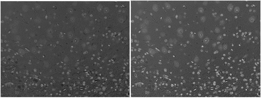
But all this is just setting the stage for the real topic I’m writing about today, which is color transformations. See, a fact that I glossed over pretty quickly above is how to create a segmentable grayscale image from a color one. The most obvious approach: average the RGB channels. What a way to lose a lot of information! Look at these two images. The neurons in the background are hard enough to see in the color image, but at least their blue tinge helps give them away; in the grayscale they are really faint.
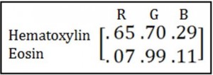
So I went hunting around in the literature for better things to do with my RGB channels than just average them. The first thing I found is Ruifrok’s seminal 2001 piece introducing color deconvolution, which recently celebrated its 18 billionth citation. The basic idea is this. You know the optical densities in each color channel of each individual stain you’re using and you put them in a matrix, e.g.:
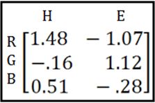
Then you take the inverse* of that matrix:
(*more on this “inverse” business later)
Then you multiply each pixel in your image by the inverse, and if you had n stains you get out n grayscale images, one representing each stain’s contribution to the original image:
In the above example, a particular pixel with R = 160, G = 251, B = 68 is deconvoluted to give a value of ~232 for hematoxylin and ~89 for eosin. By doing this to every pixel you would come up with two grayscale images, one for each stain.
Brilliant! Look at how much more the neurons pop out from the background when I use color deconvolution than when I simply average the channels:
(left: RGB channels averaged and inverted. right: The hematoxylin stain image obtained by color deconvolution.)
*Note on matrix inversion. My understanding is that for color deconvolution, you actually only need the right inverse, and thus it can be done with any matrix size, a fact which Ruifrok sidesteps by happening to choose an example with 3 stains which conveniently gives you a 3×3 matrix of which you can take a true inverse. After reading the paper I was a bit confused on this point, but CellProfiler’s implementation of this concept (the UnmixColors module) simply does this to get the inverse matrix:
return np.array(absorbance_matrix.I[:,idx]).flatten()
They use numpy‘s matrix.I operation, which does work on non-square matrices and indeed it turns out CellProfiler will let you unmix colors for any number of stains.
OK, so color deconvolution was a big help and my machine learning algorithm was able to do a bit better on the hematoxylin grayscale image than the averaged grayscale image:
(right: This segmentation achieved a Rand index of .88, a bit better than by averaging to grayscale. it has fewer extra objects but still a lot of splits).
But it’s still full of splits and mergers. In part, I’ve got some work to do on the machine learning approach–the scoring metric could use some work, and I may not have varied the continuous-valued settings widely enough or finely enough. But I also found some more recent work that takes color transformations several steps further in terms of complexity:
The angle here is they use a ground truth classifying the image into two classes (nucleus and extracellular) in order to machine learn an optimized most discriminant color space (MDC) which they then use for segmentation. They also do a lot of heavy duty post-processing, using radial symmetry and concavity detection to find and split touching cell clumps. If you like matrices, you’ll love this paper. The performance they show their algorithm achieving is certainly better than anything I’ve gotten so far! This may be a new angle to explore.


