Power analysis for mouse studies using the t test vs. log-rank test
In my last post I looked at the Student’s t test vs. log-rank test for determining significance in survival differences between control and treatment groups in a mouse study. You can argue that each test is better in particular circumstances, and which one you use might depend on your data.
That’s kind of a lame answer, though, especially if you’re still designing your study and you want to know how many mice you need. Power analysis for these two tests might give you a pretty different answer.
First let’s talk through power analysis at a concept level. Four variables are related to one another: α (false discovery rate), 1-β (power; β=false negative rate), n (sample size), and θ (effect size). There’s a PV=nRT sort of relationship between these four: any three determine the other one. Here I’m assuming effect size is expressed in standard deviations (e.g. the effect size you’re looking for could be “the treatment increases mean survival by 0.5 standard deviations” thus θ=Δ/σ; otherwise you should consider Δ = μtreatment-μcontrol (absolute effect size e.g. “increase survival by 10 days”) and σ2 (variance) as two separate inputs.
To get started, how do we do a power analysis for these tests? For the t test you can use a simple built-in R function, power.t.test. I’m going to digress here for a bit because I feel the need to understand any tool I’m going to use rather than just black boxing it. Something I love about R is that you can just type a function’s name at the prompt to see its source code. Here is what power.t.test looks like:
function (n = NULL, delta = NULL, sd = 1, sig.level = 0.05, power = NULL,
    type = c("two.sample", "one.sample", "paired"), alternative = c("two.sided",
        "one.sided"), strict = FALSE)
{
    if (sum(sapply(list(n, delta, sd, power, sig.level), is.null)) !=
        1)
        stop("exactly one of 'n', 'delta', 'sd', 'power', and 'sig.level' must be NULL")
    if (!is.null(sig.level) && !is.numeric(sig.level) || any(0 >
        sig.level | sig.level > 1))
        stop("'sig.level' must be numeric in [0, 1]")
    type <- match.arg(type)
    alternative <- match.arg(alternative)
    tsample <- switch(type, one.sample = 1, two.sample = 2, paired = 1)
    tside <- switch(alternative, one.sided = 1, two.sided = 2)
    if (tside == 2 && !is.null(delta))
        delta <- abs(delta)
    p.body <- quote({
        nu <- (n - 1) * tsample
        pt(qt(sig.level/tside, nu, lower.tail = FALSE), nu, ncp = sqrt(n/tsample) *
            delta/sd, lower.tail = FALSE)
    })
    if (strict & tside == 2)
        p.body <- quote({
            nu <- (n - 1) * tsample
            qu <- qt(sig.level/tside, nu, lower.tail = FALSE)
            pt(qu, nu, ncp = sqrt(n/tsample) * delta/sd, lower.tail = FALSE) +
                pt(-qu, nu, ncp = sqrt(n/tsample) * delta/sd,
                  lower.tail = TRUE)
        })
    if (is.null(power))
        power <- eval(p.body)
    else if (is.null(n))
        n <- uniroot(function(n) eval(p.body) - power, c(2, 1e+07))$root
    else if (is.null(sd))
        sd <- uniroot(function(sd) eval(p.body) - power, delta *
            c(1e-07, 1e+07))$root
    else if (is.null(delta))
        delta <- uniroot(function(delta) eval(p.body) - power,
            sd * c(1e-07, 1e+07))$root
    else if (is.null(sig.level))
        sig.level <- uniroot(function(sig.level) eval(p.body) -
            power, c(1e-10, 1 - 1e-10))$root
    else stop("internal error")
    NOTE <- switch(type, paired = "n is number of *pairs*, sd is std.dev. of *differences* within pairs",
        two.sample = "n is number in *each* group", NULL)
    METHOD <- paste(switch(type, one.sample = "One-sample", two.sample = "Two-sample",
        paired = "Paired"), "t test power calculation")
    structure(list(n = n, delta = delta, sd = sd, sig.level = sig.level,
        power = power, alternative = alternative, note = NOTE,
        method = METHOD), class = "power.htest")
}
I had to pore over this several times before I figured out what it was doing. The key here is this expression which determines power:
pt(qt(sig.level/tside, nu, lower.tail = FALSE), nu, ncp = sqrt(n/tsample)* delta/sd, lower.tail = FALSE)
Let me explain what the relationship here is (for a two-sample, two-sided t test):
tsampleis the number of groups: 2 for a two-sample test, 1 for a one-sample testdeltais Δ, the absolute effect size (μtreatment-μcontrol)sdis σ, the standard deviationdelta/sdis θ, the effect size in units of standard deviationsnu, the total degrees of freedom, is the number of mice (n) per group times tsamplencp, the noncentrality parameter for the t distribution, is sqrt(n/tsample)*thetasig.levelis α, the false discovery ratetsideis the sidedness of the test, i.e. 2 for 2-sidedsig.level/tsidejust adjusts to calculate based on one tail, so if alpha = .05 in a two-tailed test, you need to make sure .05/2 = .025 of the probability lies below the .025 quantile.qtis the inverse CDF of the t distribution, soqt(.025, nu, lower.tail = FALSE)gives you the t value at which 2.5% of the cumulative probability lies below that t value.ptis the CDF of the t distribution, so the overall expression gives the fraction of cumulative probability lying below the t value from the above bullet point, in a t distribution with the given non-centrality parameter.
So this is the expression if you have the other inputs and you want to determine power. R doesn’t actually have expressions to determine the other variables– instead, it uses uniroot, which is just an iterative approach to find the value that gives the specified power (like ‘goalseek’ in Excel).
So notice that in power.t.test, you put in Δ and σ as parameters and what it actually uses is delta/sd = Δ/σ = θ, the effect size in terms of standard deviations.
This is important. Power depends on variance. It really and truly does. Think of it this way: Δ = signal and σ = noise. It’s hard to see the signal of a drug’s effect through the noise of high variance in mouse phenotype.
As an example, consider Riemer 2008‘s data on curcumin in scrapie mice. Riemer tested curcumin in groups of about 17 mice, standard deviation in the control and treatment group were each about ±9 days, and let’s assume that 90% power at the α=.01 threshold was desired. This study was 90% powered to detect delays in disease onset of at least 12 days (~6% delay in onset):
> power.t.test(n=17,delta=NULL,sd=9,power=.9,sig.level=.01)

     Two-sample t test power calculation

              n = 17
          delta = 12.5691
             sd = 9
      sig.level = 0.01
          power = 0.9
    alternative = two.sided

 NOTE: n is number in *each* group
In some other studies (e.g. Cortes 2012), standard deviation for survival has been as small as ±4 days. If Riemer’s mice had such little variance, then Riemer’s study would have been 90% powered to detect changes down to about 5 or 6 days (~3% delay in onset):
> power.t.test(n=17,delta=NULL,sd=4,power=.9,sig.level=.01)

     Two-sample t test power calculation

              n = 17
          delta = 5.586265
             sd = 4
      sig.level = 0.01
          power = 0.9
    alternative = two.sided

 NOTE: n is number in *each* group
So variance matters. As it should.
My problem with power analysis for the log-rank test is that it doesn’t account for variance. I can’t claim to completely understand the reasons for this, but it seems to be steeped in the fact that hazard rates are usually modeled as exponential distributions, thus implying that the hazards themselves occur as Poisson processes. In an exponential distribution with rate λ, the expected value and the standard deviation are both just 1/λ. That’s a property of the distribution. It’s not like a normal distribution where you get to specify the mean and standard deviation separately. So the effect size (difference in rates) already includes all the information about the difference in variance.
Terry Therneau, author of the R survival package and this awesome documentation, also contributed this explanation of how to calculate power for the log-rank test, easily the most concise explanation of it on the web. I wrote a quick R function to wrap the logic he put forth:
# alpha = false discovery rate
# power = desired power
# prop = proportion of total mice in treatment vs. control group (ex. .2 for 20% v. 80%)
# hazardratio = effect size, e.g. to detect 10% delay in onset use 1.1
logrankpower = function(alpha,power,prop,hazardratio) {
    return ( ((qnorm(1-alpha/2) + qnorm(power))^2) / ((prop)*(1-prop)* log(hazardratio)^2) )
}
And it gives me some peculiar answers. I get the same 341 that he states, so I think I wrote the function correctly. This power analyis would say that in order to have 90% power at the α=.01 threshold to detect a 6% change in age at death in scrapie mice with 50/50 treatment/control mice, you would need to observe 17,529 deaths of mice:
> logrankpower(.01,.9,.5,1.06)
[1] 17529.57
Whereas, as shown above, the t test says you’ve got that amount of power with 34 mice (17 per group). But if you’re modeling the deaths as an exponential distribution, and the average age of onset is 200 days, then the exponential distribution requires that the standard deviation also be 200 days. Which is clearly not the case.
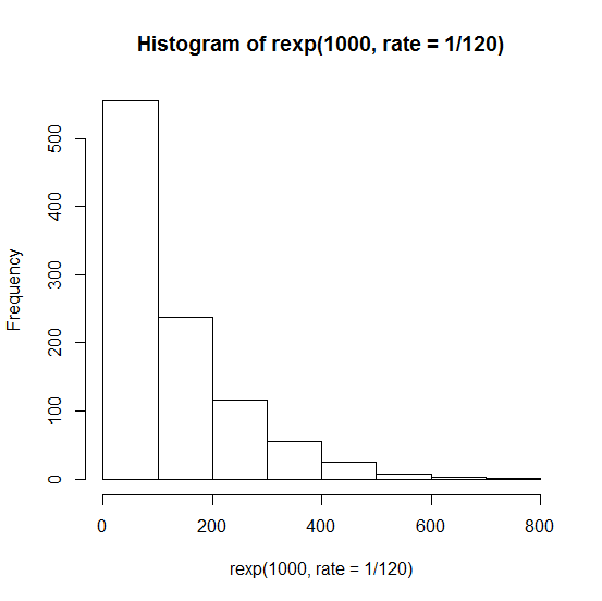
And neither is it the case that the ages at death of these mice follow an exponential distribution (where probability density is always highest at zero, no matter how low the rate) which would look like this:
hist(rexp(1000,rate=1/120))
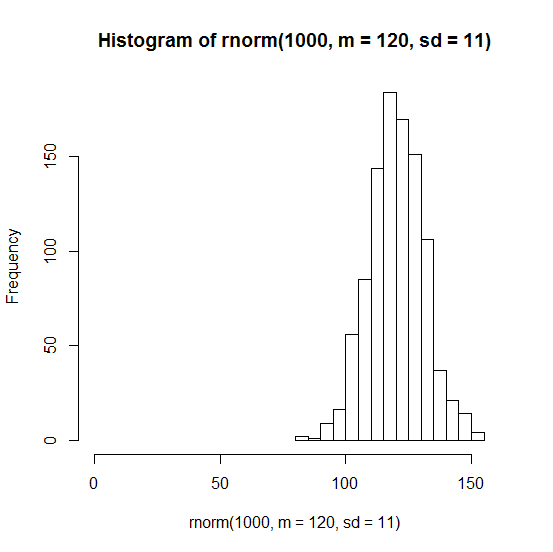
Instead it looks much more like a normal distribution:
hist(rnorm(1000,m=120,sd=9),xlim=c(0,150))
Remember that the Poisson process is used to model rare events, whereas mice infected with scrapie die very reliably. The exponential distribution might be perfect for, say, clinical trials of drugs that lower risk of cardiovascular disease, where the “event” is someone having a heart attack, and (1) most people in the study won’t have one whether or not they get the drug, purely by chance, and (2) those who do have heart attacks might have them right away; there is no “incubation period”.
Now, the log-rank test itself (as far as I can tell) does not exactly assume an underlying Poisson model. Because it only looks at the order of events and not the absolute times, it does not incorrectly assume that the deaths of mice follow an exponential distribution like that shown in the histogram above.
But this power calculation does seem to assume that, and that’s why it gives outlandish answers like 17,529 mice.
Based on my current understanding, my thinking is that power calculations for mouse studies should be based on a t test because its assumptions—normality, equal variance that you specify, all mice reaching an endpoint (whether that’s symptom onset, death, etc.) eventually—seem to be pretty well met for prion-infected mice. If your therapeutic is so awesome that some mice make it to the end of the study with no symptoms, then you can’t really use a t test on your data, but then again, if your therapeutic is that effective, you probably won’t have any trouble establishing statistical significance anyway.


