Statistical power for bioluminescence studies
motivation
In my last post I discussed one possible study design for a therapeutic trial of anle138b in mouse models of fatal familial insomina and E200K Creutzfeldt-Jakob Disease. In the cost structure for such a study, it turned out that > 80% of the costs in the initial cost estimate were directly proportional to the number of times that the mice had to to undergo bioluminescence imaging (BLI). It occurred to me that because the age of onset in these mice is fairly variable, our study is in any case not powered to detect small changes in onset due to therapeutic treatment – for instance, my power curves showed we’d be unlikely to detect a 10% delay in onset. Given that we can only detect large effect sizes anyway, I wondered whether our power would really be diminished much by only imaging the mice once every two or three weeks instead of every week. The purpose of this post is to model how the frequency of observation affects statistical power in studies using BLI as a readout.
background
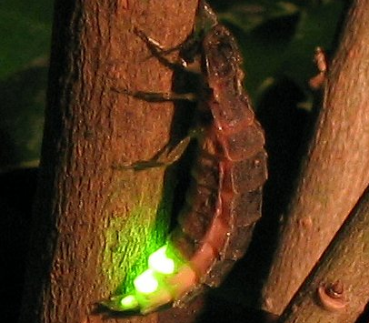
Above: Lampyris noctiluca, one of the many species that use luciferase to create bioluminescence. Wikimedia Commons image by Wofl.
Luciferase is an enzyme that breaks down the small molecule luciferin in order to release light. Some wavelengths of that light pass right through bone, such that if a luciferase transgene is expressed in the mouse brain and mice are injected with luciferin, a fancy piece of equipment called the IVIS Spectrum can quantify the amount of light.
Almost a decade ago, the development of mice with a GFAP-luc transgene made it possible to monitor upregulation of GFAP using BLI [Zhu 2004]. GFAP is a gene expressed in glial cells and it is upregulated during neurological stress, so the amount of luciferase produced in these mice is an indication of how advanced a disease is in their brain. This transgene has since become a tool for studying several neurological diseases [Cordeau 2008 (ft), Keller 2009, Watts 2011, Stohr 2012, Jany 2013]. BLI is an accurate proxy for prion replication in the brain [Tamguney 2009] and more recently it was validated as a proxy for therapeutic efficacy in a study of cpd-B as a therapeutic against RML prions [Lu & Giles 2013 (ft)].
BLI involves imaging the mice in an IVIS Spectrum at regular intervals (say, weekly), a quick (< 5 minute per mouse) process that involves injecting each mouse with 1.5 mg of luciferin (“50 ul of 30 mg/ml D-luciferin potassium salt solution” [Lu & Giles 2013 (ft)]. BLI eliminates the need for labor-intensive (read: expensive) behavioral phenotyping of mice. But it turns out that luciferin is expensive too. It’s not for lack of competition – it’s available from several commercial suppliers - Gold BioTech, PerkinElmer, Sigma, and Life at a minimum – but the best price works out to around $3 per dose. Multiply that by tens of mice and tens of weeks of imaging, and it can easily become the largest single cost in a study. Add to that the time that a technician or research assistant spends imaging the mice, which is likely to be the study’s largest labor cost, and it’s clear that reducing the number of imaging sessions could lead to potentially huge cost savings. update: we later found a better luciferin price – see our revised budget – which makes this issue less important, though the labor involved is still a good reason not to image more often than you need to.
In practice bioluminescence has been monitored either every 7 days [Tamguney 2009, Lu 2013 (ft)] 14 days [Watts 2011, Stohr 2012 Fig 1] or 21 days [Stohr 2012 Fig 3]. The endpoint in these studies was originally defined as being when a single scan reveals luminescence greater than 2e6 photons [Tamguney 2009] and more recently has been defined as the time when two consecutive scans both reveal luminescence greater than either 1e6 photons [Stohr 2012 supplement] or 7e5 photons [Watts 2011].
model
In order to model the relationship between observation frequency and power, I assume that each mouse will have onset at a particular point in time but that the onset won’t be observed until the following BLI session, so that for instance if they are monitored every Friday, then onset on a Monday won’t be noticed until four days later, and thus onset on a Monday and on a Wednesday of the same week are indistinguishable. The less frequent the imaging, the more timepoints become indistinguishable from one another.
code
First, some quick startup code:
library(sqldf) # SQL's group by is more intuitive to me than R's aggregate!
library(survival) # for log-rank test
options(stringsAsFactors=FALSE)
And then a wrapper for the simplest case of the log-rank test (from this post):
simplesurvtest = function(vec1,vec2) { # vec1, vec2: lists of survival times of mice in control and treatment groups
    days = c(vec1,vec2) # make a single vector with times for both mice
    group = c(rep(0,length(vec1)),rep(1,length(vec2))) # make a matching vector indicating control/treatment status
    status = rep(1,length(vec1)+length(vec2)) # "status" = 1 = "had an event" for all mice
    mice = data.frame(days,status,group) # convert to data frame
    return (survdiff(Surv(days,status==1)~group,data = mice)) # return log-rank test results
}
And wrappers to return p values from the t, log rank and Kolmogorov-Smirnov tests:
p_t = function(control_onset,treated_onset) {
    t_test_result = t.test(control_onset,treated_onset,alternative="two.sided",paired=FALSE)
    return (t_test_result$p.value)
}

p_lrt = function(control_onset,treated_onset) {
    lrt_test_result = simplesurvtest(control_onset,treated_onset) # call wrapper function for simple survival test
    lrt_p_value = 1 - pchisq(lrt_test_result$chisq, df=1) # obtain p value from chisq statistic by taking 1 - CDF(chi at 1 degree of freedom)
    return (lrt_p_value)
}

p_ks = function(control_onset,treated_onset) {
    ks_test_result = ks.test(control_onset, treated_onset)
    return(ks_test_result$p.value)
}
And a function to handle rounding up the day of onset to the next day of BLI observation:
# rounds a value up to the next time it would be observed, e.g. if monitoring every 7 days, gliosis at day 50 is not noticed until day 56
roundup = function(rawvalue, interval) {
    return ( (rawvalue %/% interval + 1)*interval ) # %/% is integer division, which rounds down; +1 rounds up instead
}
With that, I can write this function to run simulations and determine power empirically:
# function to run n_iter simulations to determine power empirically based on how many meet the alpha threshold of significance
empirical_power = function (n_iter=1000, alpha=.05, mean_onset_control, sd_onset_control, effect_size, n_per_group, obs_freq, statistical_test) {
    empirical_power_result = 0.0
    # choose a statistical test
    if (statistical_test == "t") {
        p_func = p_t
    } else if (statistical_test == "lrt") {
        p_func = p_lrt
    } else if (statistical_test == "ks") {
        p_func = p_ks
    }
    # conduct simulation
    for (iter in 1:n_iter) {
        this_iter_result = 0
        # control onset is normal(mean,sd)
        control_onset = rnorm(n=n_per_group, m=mean_onset_control, s=sd_onset_control)
        # assume that treatment increases both the mean survival and the variance, so normal(mean*(1+effect_size),sd*(1+effect_size))
        treated_onset = rnorm(n=n_per_group, m=mean_onset_control*(1+effect_size), s=sd_onset_control*(1+effect_size))

        # detect cases where roundup() makes data constant, and handle separately lest they throw errors in statistical test functions
        if ( length(unique(roundup(control_onset,obs_freq))) == 1 & length(unique(roundup(treated_onset,obs_freq))) == 1 ) {
            # if control == treated then the correct answer is NO difference
            if (roundup(control_onset,obs_freq)[1] == roundup(treated_onset,obs_freq)[1]) {
                this_iter_result = 0
            } else { # if control <> treated then the correct answer is YES there is a difference
                this_iter_result = 1
            }
        } else { # normal cases where data are not constant
            this_iter_result = (1 * (p_func(roundup(control_onset,obs_freq),roundup(treated_onset,obs_freq)) < alpha))
        }
        empirical_power_result  = empirical_power_result + this_iter_result * 1/n_iter
    }
    # return power
    return (empirical_power_result)
}
Here’s one example call which asks the following question. If control onset is 365 ± 30 days and the effect of a drug is a 10% (so ~36 day) delay in onset, what is the power to detect significance using a log-rank test at the p < .05 threshold with n = 15 mice per group, monitored via BLI every 1 day, simulated over 1000 trials?
# example to illustrate use of the function
set.seed(1111)
empirical_power(n_iter=10000, alpha=.05, mean_onset_control=365, sd_onset_control=30, effect_size=.10, n_per_group=15, obs_freq=1, statistical_test="lrt")
Result: 85% power.
Note that the log-rank test is particularly slow, and 10,000 iterations takes almost 1 minute.
results with some specific examples
Next we can ask how that answer depends on how often we monitor the mice. Would checking them every 7 days, 14 days or 21 days give us less power than checking every day?
# power with monitoring every 7, 14 or 21 days
set.seed(12345)
empirical_power(n_iter=10000, alpha=.05, mean_onset_control=365, sd_onset_control=30, effect_size=.10, n_per_group=15, obs_freq=7, statistical_test="lrt")
empirical_power(n_iter=10000, alpha=.05, mean_onset_control=365, sd_onset_control=30, effect_size=.10, n_per_group=15, obs_freq=14, statistical_test="lrt")
empirical_power(n_iter=10000, alpha=.05, mean_onset_control=365, sd_onset_control=30, effect_size=.10, n_per_group=15, obs_freq=21, statistical_test="lrt")
Amazingly, no. The results for these three are 85.85%, 85.08%, and 84.63% – all well within a standard error of each other (try re-running with a different random seed and you’ll see variability from 84 to 86%). So basically: no power is lost by checking the mice only every third week compared to checking them every single day.
And even more astonishingly, this is true not just within this narrow range of 7 – 21 day intervals – you lose only a bit of power by going up to even 50 day intervals. Here’s a demonstration of that. I calculate power for every possible n-weekly interval, i.e. doing BLI every week, every other week, every third week … every 57th week.
set.seed(12345)
obs_freqs = c(seq(7,399,7))
pwrs = vector(mode="numeric")
for (obs_freq in obs_freqs) {
    pwrs = c(pwrs, empirical_power(n_iter=10000, alpha=.05, mean_onset_control=365, sd_onset_control=30, effect_size=.10, n_per_group=15, obs_freq=obs_freq, statistical_test="lrt"))
}
conditions = cbind(alpha=.05, mean_onset_control=365, sd_onset_control=30, effect_size=.10, n_per_group=15, statistical_test="lrt")[1,]
plot(obs_freqs,pwrs,type='l',lwd=3,col='red',ylim=c(0,1),xlab='BLI observation frequency',ylab='power',main='Power as a function of BLI observation frequency',sub=print_vars(conditions), cex.sub=.6)
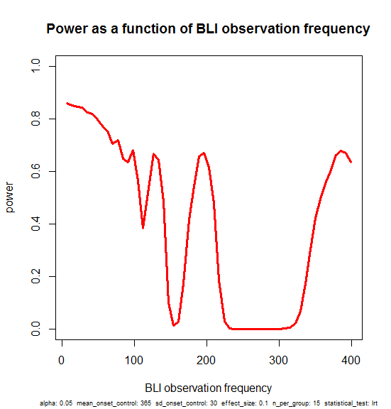
Here’s a narrative interpretation of this plot. You start with ~85% power if you monitor the mice every week, and as you space the intervals out more and more you lose just a bit of power, dropping to 80% if you only check at 50 day intervals.
But it’s not monotonic. There are spikes at 77, 98, 196 and 399 days. These should be considered as artificial. In the particular example I’ve set up, the control mice have onset around day 365 and the treated mice have onset around day 401. If the observation frequency is a divisor of some number right in the sweet spot where most of the control mice have had onset and most treated mice have not, then you can still get a significant result even though you’re doing very few observations (77*5 = 385, 98*4 = 392, 196*2 = 392, 399*1 = 399).
Those spikes, though artificial in a way, do reflect a true fact: if you are confident about the time of onset of control mice, you could design an experiment where you just keep the mice until that timepoint, then check them all histopathologically (no need to even bother with BLI) and do a Fisher’s exact test or similar to test whether more of the control mice than treated mice exhibit gliosis. Monitoring BLI only once, at 400 days, is equivalent to doing that. Here’s an example that illustrates this:
set.seed(12345)
n_per_group = 15
mean_onset_control = 365
sd_onset_control = 30
effect_size = .10
control_onset = rnorm(n=n_per_group, m=mean_onset_control, s=sd_onset_control)
treated_onset = rnorm(n=n_per_group, m=mean_onset_control*(1+effect_size), s=sd_onset_control*(1+effect_size))
hist(rbind(control_onset,treated_onset),beside=TRUE,col=c('red','green'))
control_onset
treated_onset
roundup(control_onset,400)
roundup(treated_onset,400)
t.test(control_onset,treated_onset) # result: 366 vs. 405 days, p = .001
fisher.test(rbind(table(roundup(control_onset,400)),table(roundup(treated_onset,400)))) # result: p = .014
In this particular example, the t test you could do on the exact onset days, if you monitored BLI every day, would give you 39-day difference in onset (366 vs. 405 days) at p = .001. If you monitor only at day 400 and day 800, you discover that 14 of 15 control mice have onset by day 400 while only 8 of 15 treated mice have onset by day 400. A Fisher’s exact test on these values gives you p = .014.
So, amazingly, even monitoring for gliosis just once really can give you a significant result, if you know enough to pick the right date to check. But that’s a gamble – in practice, we don’t know exactly when onset will occur, and there are big troughs of zero power in between the spikes, so better not to risk it. Also, part of the point of doing BLI is not just to know if there is a statistically significant difference in survival between treated and control mice, but also to quantify how large that difference is. A Fisher’s exact test can’t tell you a percentage delay in onset.
How, then, does observation frequency affect our ability to quantify the delay in onset?
set.seed(12345)
n_per_group = 15
mean_onset_control = 365
sd_onset_control = 30
effect_size = .10
obs_freqs = c(seq(7,399,7))
results=data.frame(obs_freq=numeric(),iteration=integer(),onsetdiff=numeric())
for (obs_freq in obs_freqs) {
    for (i in 1:100) {
        control_onset = rnorm(n=n_per_group, m=mean_onset_control, s=sd_onset_control)
        treated_onset = rnorm(n=n_per_group, m=mean_onset_control*(1+effect_size), s=sd_onset_control*(1+effect_size))
        onsetdiff = mean(roundup(treated_onset,obs_freq)) - mean(roundup(control_onset,obs_freq))
        results = rbind(results,c(obs_freq,i,onsetdiff))
    }
}
colnames(results)=c("obs_freq","iteration","onsetdiff")
plot(results$obs_freq+runif(n=dim(results)[1],min=-3,max=3),results$onsetdiff,pch=16,cex=.6,xlab='observation interval',ylab='Nominal difference in onset',
     main='Variability in estimated delay in onset vs. observation frequency',cex.main=.8,col='#999999')
abline(h=36.5,col='#000000')
abline(h=0,col='red')
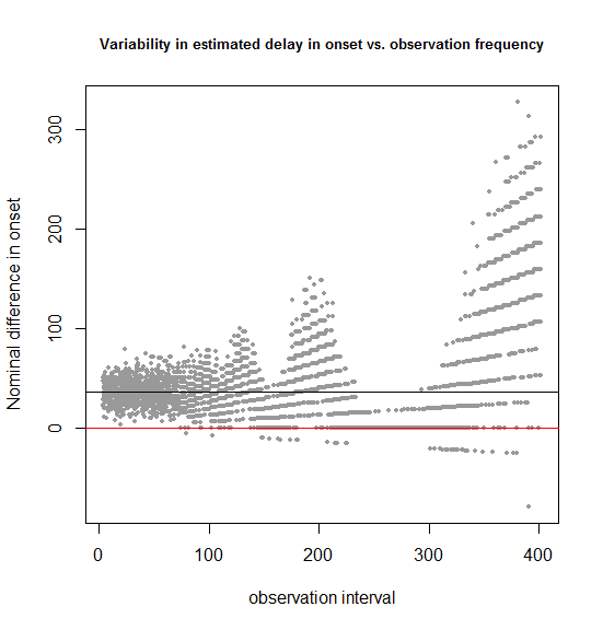
In this simulated example, we know that the true delay in onset is 36.5 days (shown by the black horizontal bar). The above code considers observation intervals of 7, 14, 21… 399 days and runs 100 simulations for each. The dispersion of the estimated difference in onset around the true value looks pretty constant for observation intervals up to 50 or 70 and then begins to balloon.
Notice also the shape of the dispersion. It begins as a cloud at the far left, where you have frequent observations, but turns into discrete streaks starting around 70 days. That’s because once the observation intervals are larger than the dispersion in the true data – the times of onset in the mice – your beautiful ratio-level data is essentially converted to categorical data. For instance, as shown in the previous example, testing only once at 400 days is equivalent to asking “how many more treated than control mice had onset by 400 days?”, and there are only 16 possible answers to that: 0, 1, 2, 3, … 15.
Another interesting point about this plot is just how few points lie below the x axis. For instance, in the 0-100 day range, there are zero simulations in which a negative delay in onset is observed. In other words, though in this case we may have limited (60-85%) power to detect a statistically significant delay in onset in the treated group, we’re overwhelmingly likely to see a nominal delay in onset.
Finally, one technical aside about this plot: to prevent dots from overlapping one another and obscuring each other’s density, I added uniformly distributed noise to each x value with +runif(n=dim(results)[1],min=-3,max=3) – this is one of my favorite R tricks.
Now, just because we can’t see an increase in dispersion over the 1-100 day range in the plot above doesn’t mean it’s not there. So I plotted the standard deviation in the estimate of delay in onset from 100 simulations at each observation frequency:
# we can't see an increase in dispersion on the plot - now let's be more formal.  *does* variance increase with larger obs_freq?
sdvals = sqldf("select obs_freq, variance(onsetdiff) variance from results group by 1 order by 1;")
m = lm(variance ~ obs_freq, data = subset(sdvals, obs_freq < 100))
summary(m)
conditions = cbind(alpha=.05, mean_onset_control=365, sd_onset_control=30, effect_size=.10, n_per_group=15)[1,]
plot(sdvals$obs_freq, sqrt(sdvals$variance),type='l', lwd=3, col='orange', main='Dispersion in estimate of delay in onset vs. observation frequency', xlab='observation interval', ylab='standard deviation in estimate', cex.main=.8, sub=print_vars(conditions), cex.sub=.6)
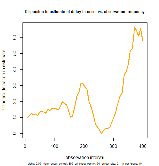
And the result is that yes, variance does increase a bit – there seems to be a positive slope, even in the 0-100 range on the x axis. But it’s subtle. And of note: the y-intercept is ~10. This reflects the fact that with a 36.5 day delay in onset (signal) on a 30 day standard deviation in onset (nosie), there is already a 10 day standard deviation in the estimates of delay in onset that you might get experimentally, even if you tested the mice with BLI every single day. Against this background level of variability, performing less frequent observations doesn’t really make the estimate that much worse. The standard deviation rises from a baseline of 10 to only about 12 by the time you get to 50-day intervals.
So yes, our ability to estimate the delay in onset is impaired a bit by observing the mice less frequently, but within a reasonable range (up to once every month or two) it’s really not that much worse than if you performed BLI every day. Or phrased differently, the vast majority of experimental error is built into the experiment by the variability of the mouse model itself, and only < 20% is due to the infrequency of observations, unless you observe even less frequently than about once in 50 days.
more general results
Everything above was just one example with very specific parameters. How generalizable is it? Can we draw any conclusions about when it is okay to save money by performing BLI less frequently versus when it really hurts you?
To answer these questions I wanted to run my simulations over a wide space of possible scenarios, so I submitted this R script to run overnight, and got this output. Note – the script I ran has a lot of other random stuff in it since I was still figuring this all out, but I left it unedited so that it accurately reflects what created the output file. The important part of the script is just this nested loop:
# Now vary the obs_freq and see how it matters.
set.seed(12345)

# fixed vars
#statistical_test = "t"
alpha = .05
mean_onset_control = 365
n_per_group = 15
n_iter = 10000
# iterable vars
obs_freqs = c(1,7,14,21,30,60,90)
effect_sizes = c(3.5/365,7/365,14/365,21/365,30/365,.1,.3,.5,.7,1.0,1.5,2.0)
sd_onset_control_vals = c(1,3,7,14,21,30,60,90,150)
statistical_tests = c("t","lrt","ks")
results = data.frame(sd_onset_control = numeric(), effect_size=numeric(), obs_freq=numeric(), statistical_test=character(), pwr=numeric())
for (statistical_test in statistical_tests) {
    for (obs_freq in obs_freqs) {
        for (effect_size in effect_sizes) {
            for (sd_onset_control in sd_onset_control_vals) {
                pwr = empirical_power(n_iter=n_iter, alpha=alpha, mean_onset_control=mean_onset_control, sd_onset_control=sd_onset_control, effect_size=effect_size, n_per_group=n_per_group, obs_freq=obs_freq, statistical_test=statistical_test)
                results = rbind(results, c(sd_onset_control, effect_size, obs_freq, statistical_test, pwr))
            }
        }
    }
}
colnames(results) = c("sd_onset_control","effect_size","obs_freq","statistical_test","pwr")
results

write.table(results,'biolum-power-sim-results-10000.txt',sep='\t',row.names=FALSE,col.names=TRUE,quote=FALSE)

# bsub.py long 160:00 "R CMD BATCH bioluminescence-power-sim.r"
# For 10K iterations each this took ~ 6 hours
I then set up to analyze the resulting data. First off, I was curious to see how much of the variation in power over the conditions I had set up could be explained by a simple linear model of effect size, sd, observation frequency and which statistical test was used.
simres = read.table('biolum-power-sim-results-10000.txt',sep='\t',header=TRUE)

m = lm(pwr ~ sd_onset_control + effect_size + obs_freq + statistical_test, data = simres)
summary(m)
# R^2 = .46

m = lm(pwr ~ sd_onset_control * effect_size * obs_freq * statistical_test, data = simres)
summary(m)
# R^2 = .53
Only 46% can be explained in an additive linear model, and 53% with interaction terms. Power is a funny nonlinear beast. All the coefficients were significant and had their expected signs: higher SD and less frequent observations are bad for power, larger effect sizes are good for power. Log-rank and t test are more powered than the KS test.
Call:
lm(formula = pwr ~ sd_onset_control + effect_size + obs_freq +
    statistical_test, data = simres)

Residuals:
     Min       1Q   Median       3Q      Max
-0.61323 -0.27961  0.00747  0.29927  0.58923

Coefficients:
                      Estimate Std. Error t value Pr(>|t|)
(Intercept)          0.5715293  0.0153931  37.129  < 2e-16 ***
sd_onset_control    -0.0025059  0.0001374 -18.238  < 2e-16 ***
effect_size          0.3993109  0.0102772  38.854  < 2e-16 ***
obs_freq            -0.0022484  0.0002184 -10.294  < 2e-16 ***
statistical_testlrt  0.0837661  0.0159002   5.268 1.51e-07 ***
statistical_testt    0.0795741  0.0159002   5.005 6.03e-07 ***
---
Signif. codes:  0 ‘***’ 0.001 ‘**’ 0.01 ‘*’ 0.05 ‘.’ 0.1 ‘ ’ 1

Residual standard error: 0.3091 on 2262 degrees of freedom
Multiple R-squared: 0.4672,     Adjusted R-squared: 0.466
F-statistic: 396.7 on 5 and 2262 DF,  p-value: < 2.2e-16
Next I wanted to ask how much power was lost by having observations less frequent than once per week, compared to the power for weekly observations. I joined the data to itself in SQL and linearly modeled the relationship between the difference in power and the other variables:
# join to see how power is lost with less frequent observations
sql_query = "
select   s7.sd_onset_control, s7.effect_size, s7.statistical_test, so.obs_freq, s7.pwr pwr7, so.pwr pwro, s7.pwr - so.pwr pwrdiff
from     simres s7, simres so
where    s7.sd_onset_control = so.sd_onset_control
and      s7.effect_size = so.effect_size
and      s7.statistical_test = so.statistical_test
and      s7.obs_freq = 7
and      so.obs_freq > 7
;
"
compare7 = sqldf(sql_query)

m = lm(pwrdiff ~ obs_freq + sd_onset_control + effect_size, data = compare7)
                   # Estimate Std. Error t value Pr(>|t|)
# (Intercept)       0.1190553  0.0121145   9.828   <2e-16 ***
# obs_freq          0.0020599  0.0001959  10.516   <2e-16 ***
# sd_onset_control -0.0013645  0.0001172 -11.647   <2e-16 ***
# effect_size      -0.1090742  0.0087633 -12.447   <2e-16 ***
#Multiple R-squared: 0.1989,     Adjusted R-squared: 0.1974
This simple model explained about 20% of variance in power lost. But I was pretty sure the interaction between these variables would be much more interesting than any of the variables themselves. First I browsed the list of cases where we went from almost 100% power to almost 0% power:
compare7[compare7$pwrdiff > .90,]
And every entry on the list was a case with an SD of 1 – 7 days, a small effect size (≤ 36.5 days) and an observation frequency larger than the effect size. No surprises here: if your observations are less frequent than the difference between the treated and control data points, you’ll have no power. But this is only a loss of power when the SD is so small that you would have been able to see the difference if only you’d imaged more frequently.
Based on this I hypothesized that what determines loss of power is the relationship between the SD, the observation frequency and the absolute effect size (in days, as opposed to relative effect size in % as I originally had it).
I therefore created a column for absolute effect size, and converted the difference in power to a loss in power:
compare7$effect_size_abs = compare7$effect_size * 365
compare7$pwrloss = -compare7$pwrdiff # set as a negative number so that the color scheme makes more sense in image()
compare7$pwrloss[compare7$pwrloss > 0] = 0 # consider only loss, not gain, of power
And I sought to plot power loss (compared to 7 day observations as a benchmark) against absolute effect size and observation frequency, using color as a third dimension. Here’s the plot for power loss with biweekly observations as opposed to weekly.
# image() plot of power lost vs. SD vs. absolute effect size, given an observation frequency of 14 days as compared to 7 days benchmark
temp1 = compare7[compare7$obs_freq==14 & compare7$statistical_test=="lrt",c("effect_size_abs","sd_onset_control","pwrloss")]
temp2 = acast(temp1, formula = effect_size_abs ~ sd_onset_control, value.var="pwrloss")
image(1:dim(temp2)[1],1:dim(temp2)[2],temp2,xaxt='n',xlab='Effect size (days)',yaxt='n',ylab='SD of onset in controls (days)',main='Loss in power with 14-day observation frequency')
for (i in 1:dim(temp2)[1]) {
  for (j in 1:dim(temp2)[2]) {
    text(i,j,labels=formatC(temp2[i,j],digits=2,format="f"),cex=.5)
  }
}
axis(side=1,at=seq(1,dim(temp2)[1],1),labels=format(as.numeric(rownames(temp2)),digits=1),cex.axis=.6,las=2)
axis(side=2,at=seq(1,dim(temp2)[2],1),labels=format(as.numeric(colnames(temp2)),digits=1),cex.axis=.6,las=2)
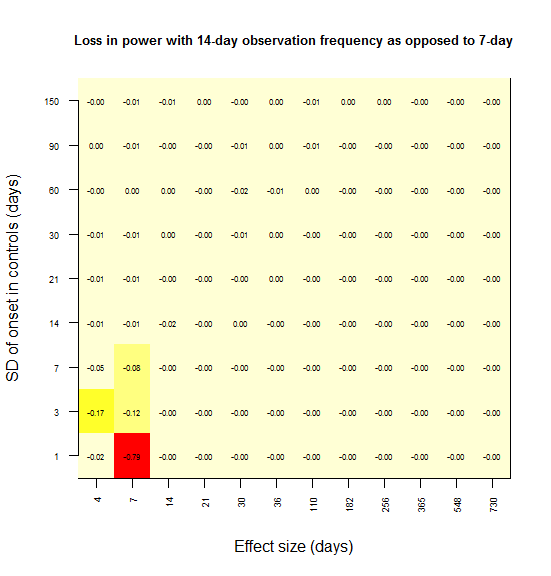
In most grid cells, no power at all is lost. A substantial amount of power is lost only in the lower left corner – for instance, there is a 79% loss in power if the effect size is 7 days and the SD is 1 day (the red square). Here’s what I interpret that lower left corner as representing:
Power is lost only when the observation interval is larger than both the effect size and the SD.
To rationalize this, consider the following. In the upper left, the SD is larger than the effect size, and so you never had any power to start with; there is no power to lose. In the lower right, the effect size is so large that you’re saturated with 100% power – you won’t miss this effect. As you move towards the upper right, both the effect size and SD are large, so coarsely detecting the difference in distributions is good enough – precision down to the level of a week is not important.
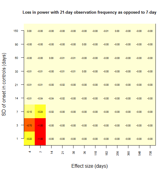
When I create the same plot for power lost at 21 days vs. 7 days, the effect is consistent with this interpretation:
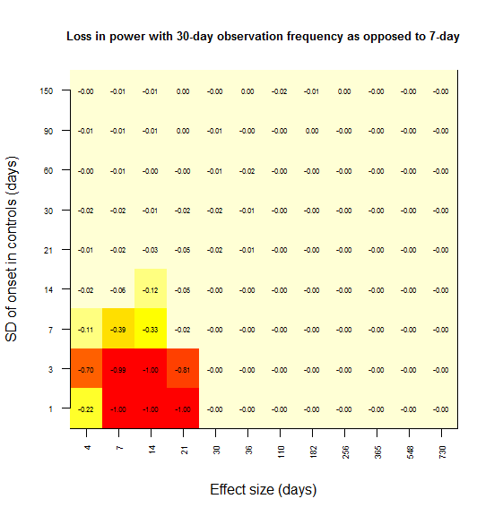
And same with 30 days:
And 60:
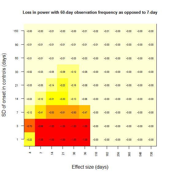
(If/when I do this over again I’ll choose regular intervals for the effect sizes and SDs that I simulate so that the x and y axes are linear.)
discussion
All of the evidence presented here suggests that doing BLI imaging less frequently than once per week only leads to a loss of power in very specific circumstances. The only time when more than 1 or 2% power is lost is when both the effect size (in days) and the standard deviation in onset are less than the observation frequency. For instance, if you image only once per month, you only lose power in cases where the effect of a drug treatment is less than a one month delay and the standard deviation in the ages of onset of the mice is less than one month.
One interpretation is that there isn’t much point in performing BLI at intervals any smaller than either the standard deviation in the mice, or the effect size (in days) that you estimate your study is powered to detect.
As a real application, consider this possible study design for anle138b. We don’t know for certain the standard deviation in age of onset of gliosis in the FFI mice, though I argued it might well be more than 30 days. We also don’t know the effect size we expect, though if anle138b’s therapeutic effectts against RML are any guide (and I wish they were!), it could easily be 30%, which would be 4 months’ delay in onset.
If we assume the standard deviation of onset in FFI mice is at least 30 days, then the conclusion from this post is that imaging weekly would provide essentially no marginal statistical power for our study compared to imaging monthly. And, as argued in one example above, imaging only once a month would also not have much impact on our ability to estimate the number of days of delay in onset.
Less frequent imaging, then, is a really good deal. In the cost structure we outlined, imaging monthly as opposed to weekly would cut the direct costs by more than half, from $20,000 to $9,000. All that for basically no loss in power.
outstanding issues
Here are a few other considerations this analysis does not address:
- Basing the measured “onset” on the first single BLI measurement above threshold vs. requiring two consecutive measurements to be above a threshold. Intuitively, it seems that imaging every 30 days and requiring 1 measurement above threshold should be equivalent to imaging every 14 days and requiring 2 measurements above threshold. But I’m not certain that’s correct, and I haven’t modeled it here.
- Many of the published BLI studies see a jagged pattern of BLI photons over time [e.g. red line in Watts 2011 Fig 2]. In some cases [e.g. orange line in Stohr 2012 Fig 1] the difference between times is far larger than the variance within any one time. Does anyone know what causes this week-to-week variation?
- I haven’t explicitly modeled the measurement error in the BLI process itself, i.e. the noise in the number of photons measured.
- It’s possible that in the FFI mice, for instance, the gliosis is more gradual/subtle and there will not be a single obvious inflection point. If so, it might prove more appropriate to compare the slopes of the BLI curves using an ANCOVA or something like that. I haven’t modeled how the power of such a test would be affected by less frequent observations.
I welcome any suggestions or critiques – including suggestions of how to incorporate the above ideas.

About Eric Vallabh Minikel
Eric Vallabh Minikel is on a lifelong quest to prevent prion disease. He is a scientist based at the Broad Institute of MIT and Harvard.