Counts vs. FPKMs in RNA-seq
motivation
Most of the time, the reason people perform RNA-seq is to quantify gene expression levels. In theory, RNA-seq is ratio-level data, and you should be legitimately able to compare Gene A in Sample 1 vs. Sample 2 as well as Gene A vs. Gene B within Sample 1.
There are two main ways of measuring the expression of a gene, or transcript, or whatever, in RNA-seq data:
- counts are simply the number of reads overlapping a given feature such as a gene.
- FPKMs or Fragments Per Kilobase of exon per Million reads are much more complicated. Fragment means fragment of DNA, so the two reads that comprise a paired-end read count as one. Per kilobase of exon means the counts of fragments are then normalized by dividing by the total length of all exons in the gene (or transcript). This bit of magic makes it possible to compare Gene A to Gene B even if they are of different lengths. Per million reads means this value is then normalized against the library size. This bit of magic makes it possible to compare Gene A in Sample 1 to Sample 2 even if Sample 1′s RNA-seq library has 60 million pairs of reads and Sample 2′s library has only 30 million pairs of reads.
(In fact, as this post will show, there are more differences between the two methods than just these – I’ll return to this in the conclusion.)
To my mind, normalizing by exonic length and library size seems like a no-brainer, so I use FPKMs and had never understood why anyone would use counts. But if you really want to defend your analysis you need to be able to answer any question with “Yes, I tried that and here’s what I found,” and so I wanted to repeat my analysis using counts. Meanwhile, a colleague who’s into counts told me that FPKMs apply too much normalization, glossing away some of the difference between one sample and another. Why would that be the case? I decided as long as I was going to repeat my analyses using counts I might as well do a side-by-side comparison with FPKMs in order to really understand how the behavior differs.
To compare the two, I turned to my go-to RNA-seq dataset: Human BodyMap 2.0. For the purposes of this exercise, I’ll look only at known transcripts.
how to calculate FPKMs
I previously calculated FPKMs for the Human BodyMap 2.0 data, and here is the bash script I used to do it. I used Cufflinks [Trapnell 2010].
how to calculate counts
You can calculate counts using bedtools multicov, but you need a transcript annotation file in BED format to tell bedtools where to look – unlike Cufflinks with the -N 1 setting, multicov is not going to go out and discover novel transcripts for you. To make the counts directly comparable to the FPKMs I calculated earlier, I wanted to use that same transcript annotation file and convert it from GTF to BED format.
Right off the bat, things get complicated. I noticed that the original transcript annotation file has one row per every combination of one transcript with an exon or coding sequence or start or stop codon. Consider PRNP, which only has two exons (exon 1 is the 5′ UTR and exon 2 is the coding sequence and 3′UTR) and really only one transcript – there are no major splicing variations I’m aware of. It has 18 rows in this file.
cat Homo_sapiens.GRCh37.70.gtf | grep PRNP | wc -l
18
That’s because 4 distinct versions of PRNP somehow made it into Ensembl’s database as distinct transcripts – some blatantly have the wrong coding sequence coordinates (the real coding sequence ends at chr20:4680625 in hg19).
In any case, if it’s that bad for PRNP you can imagine how many rows are present for genes that legitimately have a lot of splicing variants:
cat Homo_sapiens.GRCh37.70.gtf | grep "gene_name \"TTN\"" | wc -l
3393
This presents us with a problem. Now, if we wanted counts for each possible exon, we could just use the gtf2bed tool in bedops which will convert that original GTF file into a BED file, line by line:
gtf2bed < ../gtf/Homo_sapiens.GRCh37.70.gtf > ../gtf/Homo_sapiens.GRCh37.70.bed
(Run time: ~ 5 mins). But more likely our unit of analysis is transcripts or gene symbols. If we were to do counts by exon and then group by transcript or gene symbol and take the sum of exon counts, we’d be quadruple-counting each exon in PRNP and counting each exon in TTN many more times than that! What we need is to convert the GTF file to one row per, say, gene symbol, if gene symbol is our unit of analysis.
It turns out that Erik Aronesty‘s ea-utils contains a Perl script to do just that. It is named gtf2bed just like the bedops tool above, so for clarity I’ve renamed it gtf2bed_2.pl. To download and run it:
wget http://ea-utils.googlecode.com/svn/trunk/clipper/gtf2bed -O gtf2bed_2.pl
gtf2bed_2.pl Homo_sapiens.GRCh37.70.gtf gene_name > Homo_sapiens.GRCh37.70.gtf.gene_name.bed
Which takes ~1 minute. (Warning: if you’re using this post as a pipeline, note that using the resulting BED file without modification can give very nonsensical results for genes listed in multiple loci – see discussion of SNORD60 further on in this post).
If you open the resulting bed file you’ll see that the first three columns are simply the chromosome, (earliest) transcription start site and (latest) transcription end site for the gene – or in other words, the union of all transcribed sites in that gene over all possible transcripts.
Now, gtf2bed_2.pl observes very proper BED12 format and therefore does preserve the exon structure information in the form of the blockSizes and blockStarts columns. But multicov doesn’t read anything but the first three columns. Therefore when you do counts on this file we just created, you’ll be counting introns and exons alike. As far as I can tell by asking around, this is how everyone does their RNA-seq counts.
Contrast this with FPKMs, where Cufflinks will count only exonic reads and will normalize by a gene’s (or transcript’s) total exon length, if you do counts (at least according to this pipeline / unless you do other, fancier stuff) you are including intronic reads. So counts – unlike FPKMs – will be affected by how much pre-mRNA contamination (and therefore intronic coverage) you have in your libraries.
With all that said, next I ran multicov, like so:
bedtools multicov -bams GRCh37.HumanBodyMap.adipose.1.bam GRCh37.HumanBodyMap.adrenal.1.bam GRCh37.HumanBodyMap.blood.1.bam GRCh37.HumanBodyMap.brain.1.bam GRCh37.HumanBodyMap.breast.1.bam GRCh37.HumanBodyMap.colon.1.bam GRCh37.HumanBodyMap.heart.1.bam GRCh37.HumanBodyMap.kidney.1.bam GRCh37.HumanBodyMap.liver.1.bam GRCh37.HumanBodyMap.lung.1.bam GRCh37.HumanBodyMap.lymph.1.bam GRCh37.HumanBodyMap.ovary.1.bam GRCh37.HumanBodyMap.prostate.1.bam GRCh37.HumanBodyMap.skeletal_muscle.1.bam GRCh37.HumanBodyMap.testes.1.bam GRCh37.HumanBodyMap.thyroid.1.bam -bed ../gtf/Homo_sapiens.GRCh37.70.gtf.gene_name.bed > counts.bed
Which took about 50 hours of CPU time.
By the way, generating the list of BAM files for this command is annoying; this time I did it with echo -n:
for tissue in {adipose,adrenal,blood,brain,breast,colon,heart,kidney,liver,lung,lymph,ovary,prostate,skeletal_muscle,testes,thyroid}; do echo -n "GRCh37.HumanBodyMap.$tissue.1.bam "; done
The resulting file will have the original 12-column bed file created by gtf2bed_2.pl plus, in this case, 16 additional columns for each of the 16 BAMs I called counts on using multicov.
a couple of covariates
Since FPKMs are, in theory, just counts normalized by library size and transcript size, I figured I should have those two values on hand for this analysis as well. I calculated the library size as number of reads in each BAM with samtools view -c:
for tissue in {adipose,adrenal,blood,brain,breast,colon,heart,kidney,liver,lung,lymph,ovary,prostate,skeletal_muscle,testes,thyroid}
do
   bsub -q medium -W 05:00 "samtools view -c /data/HD/dataset/humanbodymap2.0/GRCh37.HumanBodyMap.$tissue.1.bam > /data/HD/dataset/humanbodymap2.0/$tissue.readcount"
done
Which takes a surprisingly long time (~30 min/BAM), hence the need to submit each one as a job.
The other covariate I wanted was the length of each gene. But which length, you ask? Using the BED file I just created, it’s easy to get the length from the earliest transcription start site to the latest possible transcription end site:
cat Homo_sapiens.GRCh37.70.gtf.gene_name.bed | awk '{print $4"\t"$3-$2}' > gene.lengths.txt
If you want the exonic length, that’s slightly tricker. Obviously, Cufflinks knows this information in some form since it’s used for normalization, so I looked back at the isoforms.fpkm_tracking file from Cufflinks and saw that indeed it has a length value for each transcript. You can pull that out like so:
cat combined/all.isoforms.fpkm_tracking | grep adipose | awk '{print $2" "$9}' > transcripts.length # $2 is Ensemble transcript ID, $9 is length
But genes.fpkm_tracking does not have this for genes, presumably since choosing one length as “the” length for a gene with multiple transcripts is awkward. With some fancier scripting and bedtools merge, you could get the length of the union of all possible exons in a gene, sort of analogous to gene.lengths.txt file we just created, which is the length of the union of all possible transcripts. But I won’t necessarily need that for today.
For the sake of argument, I also calculated straight-up average lengths for each gene symbol, crude though that is. First I grabbed gene symbols and length in bash:
cat combined/all.isoforms.fpkm_tracking | grep adipose | awk '{print $6" "$9}' > genesymbols.length # $6 is gene symbol
and then just some SQL wrapped in R:
library(sqldf)
lengths = read.table('genesymbols.length')
colnames(lengths)=c('gene_symbol','bases')
avlen = sqldf("select gene_symbol, avg(bases) avlen from lengths group by 1 order by 1;")
write.table(avlen,'genesymbols.av.length',row.names=FALSE,col.names=FALSE,quote=FALSE)
comparison
With the counts, FPKMs and covariates in hand I set out to understand how and why these measures differed from one another.
First, the boring setup stuff:
# Eric Minikel
# 2013-09-11
# CureFFI.org
# Comparing counts vs. FPKMs for the same Human BodyMap 2.0 data

setwd('c:/sci/026rplcl/hbm')
options(stringsAsFactors=FALSE)
library(reshape2)
library(sqldf)

# read in data
fpkms = read.csv('gene.matrix.csv') # see /2013/07/11/tissue-specific-gene-expression-data-based-on-human-bodymap-2-0/
counts = read.table('counts.gene_name.bed',sep='\t')
genelengths = read.table('gene.lengths.txt',sep='\t')
libsizes = read.table('readcounts.txt',sep='\t')
exoniclengths = read.table('genesymbols.av.exonic.length')
refseq = read.table('hg19.refseq.gene_.symbols.txt') # /wp-content/uploads/2013/09/hg19.refseq.gene_.symbols.txt

# make informative column names
tissue.names = c("adipose","adrenal","blood","brain","breast","colon","heart","kidney","liver","lung","lymph","ovary","prostate","skeletal_muscle","testes","thyroid")
bed12.colnames = c("chrom","chromStart","chromEnd","name","score","strand","thickStart","thickEnd","itemRgb","blockCount","blockSizes","blockStarts")
colnames(counts) = c(bed12.colnames,tissue.names)
colnames(genelengths) = c("genesymbol","length")
colnames(libsizes) = c("tissue","reads")
colnames(fpkms)[1] = "genesymbol"
colnames(exoniclengths) = c("genesymbol","length")
colnames(refseq)[1] = "genesymbol"
# double check that genes are not double counted, as we'll need 1:1 joins later
dim(fpkms)[1] == length(unique(fpkms$genesymbol)) # TRUE
dim(counts)[1] == length(unique(counts$name)) # TRUE

# melt the matrices down to 3-column relational form
fpkm_rel = melt(fpkms)
colnames(fpkm_rel) = c("genesymbol","tissue","fpkm")
count_rel = melt(counts[,c(4,13:28)]) # col 4 is "name" i.e. gene symbol, and cols 13:28 are the count values by tissue
colnames(count_rel) = c("genesymbol","tissue","count")

# join datasets together
sql_query = "
select   f.genesymbol, f.tissue, f.fpkm, c.count, gl.length glength, el.length elength, ls.reads
from     fpkm_rel f, count_rel c, genelengths gl, exoniclengths el, libsizes ls
where    f.genesymbol == c.genesymbol
and      f.tissue == c.tissue
and      f.tissue == ls.tissue
and      f.genesymbol == gl.genesymbol
and      f.genesymbol == el.genesymbol
order by 1, 2
;
"
merged = sqldf(sql_query)
Now we can ask questions.
Most basic question: are counts and FPKMs correlated? I would certainly hope so! We can ask this a couple ways. First, let’s ask this question across all gene symbol – tissue combinations.
cor.test(merged$fpkm, merged$count, method='pearson')  # rho = .006, p = 1.7e-7
cor.test(merged$fpkm, merged$count, method='spearman') # rho = .81,  p < 2e-16
This is strange. In linear space (Pearson’s correlation), the counts and FPKMs are significantly but barely correlated, with rho = .006. In rank space (Spearman’s correlation) they’re quite strongly correlated, rho = .81. What could these data possibly look like?
plot(merged$count,merged$fpkm,pch=16,xlab='count',ylab='fpkm',main='FPKMs vs. Counts across all tissue-gene combinations')
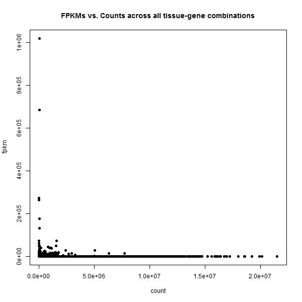
This is so extreme: in this view there appear to be basically two kinds of genes: those with some counts but ~0 FPKMs, and those with some FPKMs but ~0 counts. Amazing that we saw any correlation at all.
This is even true if we take the average value for each gene across the multiple tissues considered here:
sql_query = "
select   f.genesymbol, avg(f.fpkm) av_fpkm, avg(c.count) av_count, max(gl.length) glength, max(el.length) elength
from     fpkm_rel f, count_rel c, genelengths gl, exoniclengths el
where    f.genesymbol == c.genesymbol
and      f.tissue == c.tissue
and      f.genesymbol == gl.genesymbol
and      f.genesymbol == el.genesymbol
group by 1
order by 1
;
"
gene_avgs = sqldf(sql_query)
png('count.fpkm.gene_avgs.png',width=600,height=600)
plot(gene_avgs$av_count, gene_avgs$av_fpkm, pch=16, xlim=c(0,2e7),xlab='count',ylab='fpkm',main='FPKMs vs. Counts across all genes')
text(gene_avgs$av_count, gene_avgs$av_fpkm, labels=gene_avgs$genesymbol, pos=4, cex=.8)
dev.off()
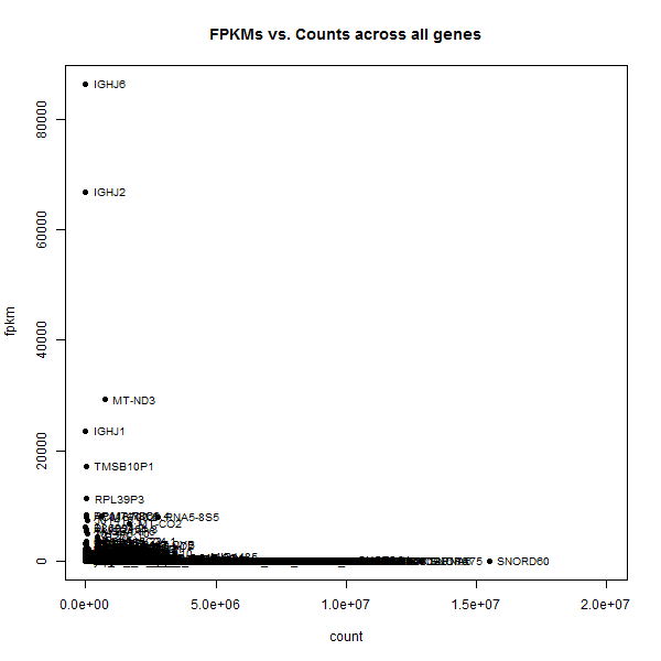
The two most extreme outliers were IGHJ6 and SNORD60, so I looked those up individually.
IGHJ6 is only 61 bp long,at chr14:106,329,408-106,329,468, so it’s no wonder that it could have low counts but high FPKMs. SNORD60, on the other hand, is also a short gene, a snoRNA of only 83 bp at chr16:2,205,024-2,205,106. So what is SNORD60′s deal?
First I looked at the raw data:
> merged[merged$genesymbol == "SNORD60",]
       genesymbol          tissue    fpkm    count    length     reads
757057    SNORD60         adipose  0.0000 14505444 204056070 230869369
757058    SNORD60         adrenal 74.5446 15192949 204056070 225117311
757059    SNORD60           blood  0.0000 21499048 204056070 245219969
757060    SNORD60           brain  0.0000 13608390 204056070 211339298
757061    SNORD60          breast  0.0000 13390021 204056070 228919690
757062    SNORD60           colon  0.0000 13993551 204056070 245132643
757063    SNORD60           heart  0.0000 12458671 204056070 242604430
757064    SNORD60          kidney  0.0000 14331012 204056070 240567067
757065    SNORD60           liver  0.0000 14009809 204056070 237551123
757066    SNORD60            lung  0.0000 17199850 204056070 239849248
757067    SNORD60           lymph  0.0000 15231013 204056070 246072774
757068    SNORD60           ovary 30.6890 17222316 204056070 242895572
757069    SNORD60        prostate 83.4049 17971399 204056070 247988054
757070    SNORD60 skeletal_muscle  0.0000 14695613 204056070 247086914
757071    SNORD60          testes  0.0000 16086969 204056070 245716717
757072    SNORD60         thyroid  0.0000 16319587 204056070 244072431
13-21 million reads but zero FPKMs in many tissues. It didn’t take long to find the source of the problem: in the BED file I used to create counts, SNORD60 is 204 Mb long:
$ cat ../gtf/Homo_sapiens.GRCh37.70.gtf.gene_name.bed | grep SNORD60
1       2205023 206261093       SNORD60 0       -       2205023 206261093       0       3       83,73,86,       0,126263247,204055984,
Which turns out to be because in the original GTF file it is listed with three exons in completely different genomic loci.
$ cat ../gtf/Homo_sapiens.GRCh37.70.gtf | grep SNORD60
1       snoRNA  exon    206261008       206261093       .       -       .        gene_id "ENSG00000252692"; transcript_id "ENST00000516883"; exon_number "1"; gene_name "SNORD60"; gene_biotype "snoRNA"; transcript_name "SNORD60.2-201"; exon_id "ENSE00002089160";
16      snoRNA  exon    2205024 2205106 .       -       .        gene_id "ENSG00000206630"; transcript_id "ENST00000383903"; exon_number "1"; gene_name "SNORD60"; gene_biotype "snoRNA"; transcript_name "SNORD60-201"; exon_id "ENSE00001498913";
10      snoRNA  exon    128468271       128468343       .       -       .        gene_id "ENSG00000199321"; transcript_id "ENST00000362451"; exon_number "1"; gene_name "SNORD60"; gene_biotype "snoRNA"; transcript_name "SNORD60.1-201"; exon_id "ENSE00001437214";
So when I ran gtf2bed_2.pl to convert this GTF to a BED file, it simply chose the lowest start base and highest end base as the endpoints of a transcript.
It proved surprisingly difficult to find some way of filtering such cases out. The histogram of gene lengths in my BED file is just as extreme as the plots earlier:
hist(genelengths$length,breaks=100,col='yellow',main="Histogram of gene lengths",xlab='Length (bp)')
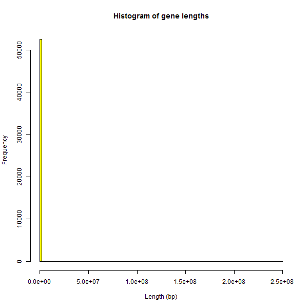
Looking for some cutoff to filter out the genes whose length is obviously an error, I Googled “longest human gene” and found DMD, which measures almost 2.3Mb. The histogram of genes ≤ 2.3Mb looks slightly better than the first histogram:
hist(genelengths$length[genelengths$length < 2300000],breaks=100,col='yellow',main="Histogram of gene lengths",xlab='Length (bp)')
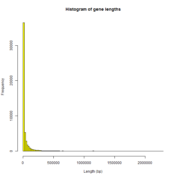
This is closer to the exponential distribution I would expect, though I suspect that there are still some erroneously long genes in this distribution too.
If this subset, of genes < 2.3Mb, is more rational and has at least eliminated some of the most outrageous errors, I would have hoped that it would be possible to explain much of the variability in counts vs. FPKMs within this subset:
m = lm(av_fpkm ~ av_count, data = subset(gene_avgs, glength < 2300000))
summary(m)
But no, linear model of FPKMs ~ counts gives an R^2 of only .008. Including gene length in the model didn’t help:
m = lm(av_fpkm ~ av_count + glength, data = subset(gene_avgs, glength < 2300000))
summary(m) # .009
And explicitly dividing counts by gene length only helped a little bit, getting us up to an R^2 of .016:
gene_avgs$av_count_over_glength = gene_avgs$av_count/gene_avgs$glength
m = lm(av_fpkm ~ av_count_over_glength, data = subset(gene_avgs, glength < 2300000))
summary(m) # .016
This dataset includes 52,686 Ensembl gene symbols, so I wondered if perhaps the data would be better behaved if we only considered the 23,705 hg19 RefSeq genes. This helped only a little bit, getting us up to an R^2 of .026:
in_refseq = gene_avgs$genesymbol %in% refseq$genesymbol
m = lm(av_fpkm ~ av_count_over_glength, data = subset(gene_avgs, glength < 2300000 & in_refseq))
summary(m) # .026
And when I went back to all gene-tissue combinations with this more limited dataset I finally got a rho of .26 for a Pearson’s correlation, and a .83 for Spearman’s.
cor.test(merged$fpkm[merged$genesymbol %in% refseq$genesymbol & merged$glength < 2300000], merged$count[merged$genesymbol %in% refseq$genesymbol & merged$glength < 2300000], method = 'pearson')
# rho = .26
cor.test(merged$fpkm[merged$genesymbol %in% refseq$genesymbol & merged$glength < 2300000], merged$count[merged$genesymbol %in% refseq$genesymbol & merged$glength < 2300000], method = 'spearman')
# rho = .83
This is still not as tight a correlation as I had hoped, considering that these two measures are supposed to be broadly measuring the same thing – gene expression – in the exact same dataset. For comparison, when I run my standard gene expression QC pipeline on RNA-seq data for different samples but called using the same pipeline, I often find a Pearson’s correlation between samples of .85 or better. Whereas here, for the same data called with two different pipelines, I get a Pearson’s of only .26. This is perhaps another unfortunate reminder of just how irreproducible gene expression findings can be. The technologies used (including the different bioinformatic pipelines) introduce more variability than is present in the underlying samples themselves.
I figured one possible explanation might be the difference between exonic length and total gene length. Here counts are assessed over total gene length, and I’ve then divided them by total gene length, whereas FPKMs are assessed over exons and normalized by exonic length. Within this relatively well-behaved set of genes ≤ 2.3Mb and in RefSeq, the correlation between total length and exonic length is still only 0.19 in linear space and 0.49 in rank space:
cor.test(gene_avgs$elength[gene_avgs$glength < 2300000 & in_refseq], gene_avgs$glength[gene_avgs$glength < 2300000 & in_refseq], method='pearson')
# rho = .19, p < 2e-16
cor.test(gene_avgs$elength[gene_avgs$glength < 2300000 & in_refseq], gene_avgs$glength[gene_avgs$glength < 2300000 & in_refseq], method='spearman')
# rho = .49, p < 2e-16
Which suggests that at least part of the problem here is just that counts, which include exons and introns, are measuring something very different than FPKMs, which include only exons.
So it seems these two metrics are just measuring something different, and getting different answers (as evidenced by the low correlation between them). That suggests that at most one of the two methods – counts and FPKMs – is suitable for comparing Gene A to Gene B. At least at a ratio level, that is. Arguably, since the Spearman’s correlation is stronger, both could be okay for ordinal-level analyses.
That’s just comparing Gene A to Gene B. But often the answer we’re looking for in our analyses is to find genes whose expression level correlates with some variable of interest – say, a genotype, drug treatment, or timepoint. Such results will be reproducible between counts and FPKMs only to the extent that counts and FPKMs for each individual gene are correlated across samples. In this case, our “samples” are the 16 different tissues in Human BodyMap 2.0. To assess how reproducible the level of each gene is across different tissues, I made a “volcano plot,” first, of Pearson’s correlations:
fpkm_mat  = acast(merged[merged$genesymbol %in% refseq$genesymbol & merged$glength < 2300000, c("genesymbol","tissue","fpkm")],  formula = genesymbol ~ tissue, value.var = "fpkm")
count_mat = acast(merged[merged$genesymbol %in% refseq$genesymbol & merged$glength < 2300000, c("genesymbol","tissue","count")], formula = genesymbol ~ tissue, value.var = "count")

pvals = numeric()
rhos = numeric()
for (i in 1:dim(fpkm_mat)[1]) {
    correl = cor.test(fpkm_mat[i,], count_mat[i,], method='pearson') # Pearson's correlation
    pvals = c(pvals, correl$p.value) # append p value
    rhos = c(rhos, correl$estimate) # append rho
}
pos.cor = rhos > 0 & pvals < .05
neg.cor = rhos < 0 & pvals < .05
plot(rhos, -log10(pvals), pch=19, main="Pearson's correlation between FPKM and counts across tissues, for each gene symbol", cex.main=.7)
points(rhos[pos.cor], -log10(pvals[pos.cor]), pch=19, col = 'blue')
points(rhos[neg.cor], -log10(pvals[neg.cor]), pch=19, col = 'red')
pearson_volcano = data.frame(rownames(fpkm_mat),rhos,pvals)
sum(pos.cor,na.rm=TRUE)/dim(fpkm_mat)[1]
sum(pvals >.05,na.rm=TRUE) / dim(fpkm_mat)[1]
sum(neg.cor,na.rm=TRUE)/dim(fpkm_mat)[1]
sum(is.na(rhos) | is.na(pvals)) / dim(fpkm_mat)[1]
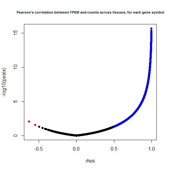
The results are much better than I expected:
| Pearson's correlation | % of genes |
|---|---|
| positive (p < .05) | 83% |
| none (p > .05) | 6% |
| negative (p < .05) | 0.01% |
| NA* | 11% |
*The NA values result from rows where either all tissues had 0 counts or all had 0 FPKMs, thus the correlation test failed.
Surprisingly, when I re-ran this with Spearman’s, the results were virtually identical (all of the numbers in the above table were within a fraction of a percent).
So for most genes, the difference between various samples’ expression levels of that gene is at least nominally reproducible between the two metrics considered here: counts and FPKMs. However, I hesitate to assign too much significance to this finding because what I’m using here as my example dataset is expression across different tissues, as opposed to different individuals. Gene expression differences between tissues are pretty large and pretty fundamental to biology, and I would expect differences between individuals to be far more subtle. Whether the same inter-individual differences show up in counts as show up in FPKMs, I can’t say in this example.
conclusions
The name “FPKM” – fragments per kilobase of exon per million reads – implies that FPKM is a measure of gene expression normalized by exonic length and library size, in contrast to raw counts. However in the course of this example I’ve realized there are several other differences between counts and FPKMs:
- When a read overlaps multiple exon definitions or multiple transcript definitions, Cufflinks makes a decision about which transcript(s) to assign the read to when it calculates FPKMs. The calculation of counts, at least in the simple pipeline I’ve presented here, is not nearly so sophistocated.
- As a result of that, counts are normally only assessed by gene symbol. If they were assessed by transcript, many reads would be double-counted (or even counted tens of times) as many genes have a multiplicity of transcripts. In comparison there are relatively few genomic loci where two distinct genes overlap.
- FPKMs only count exonic alignments, counts (at least this pipeline) include introns. A gene’s total length (including introns) is only modestly correlated with its exonic length (rho = .19), so this makes a big difference.
- Count-generating pipelines are generally not capable of transcript discovery. Instead you have to feed them a list of genomic loci with known genes (with FPKMs this is optional). It’s important to be careful that the merging of transcripts into one row per gene doesn’t create nonsensical results like we saw for SNORD60 above.
All of these differences seem to contribute to accounting for why the FPKMs and counts that I called here – on the exact same dataset – have so little correlation with each other (R^2 < .01 even after removing gene length outliers). In spite of this, the FPKMs and counts for any one gene may be somewhat more reproducible, though this analysis considered different tissues (which have enormous differences in gene expression) and not different individuals (which have subtle differences in gene expression).
Since counts and FPKMs seem to be measuring pretty different things, it’s up for debate which is the more valid measurement. I’ll put myself out there and argue a bit for FPKMs. mRNA-seq libraries are enriched for mRNAs, usually through polyA selection, thus hopefully eliminating most intronic coverage. Given that you’re using a laboratory method specifically to only get mRNAs, your pipeline should match that and only count exons. Clearly, FPKMs also represent a more sophisticated method involving assignment of reads to particular transcripts and normalization for exonic length and library size, all good things. I haven’t heard anyone deny this; the argument I’ve heard for counts has been that they’re a different measurement that may have more variability and more power for certain things. But nothing I’ve seen here has convinced me that this extra variability reflects anything meaningful that you would want to analyze.
That said, my original motivation for this post – you always want to do the analysis both ways so you can answer any questions – still stands.

About Eric Vallabh Minikel
Eric Vallabh Minikel is on a lifelong quest to prevent prion disease. He is a scientist based at the Broad Institute of MIT and Harvard.