An mRNA-seq pipeline using Gsnap, samtools, Cufflinks and BEDtools

introduction

I’m no expert on RNA-seq. I’ve analyzed RNA-seq data for just a few projects in my year at the Center for Human Genetic Research and at this point I have a pipeline that I think is worth documenting for my future reference and in case it’s useful to others. I don’t assert that this is the best way to do things – in fact, I’m pretty sure it’s not. But maybe it can be a starting point.

My tools of choice for this pipeline are Gsnap, samtools, Cufflinks, and BEDtools.

philosophy

Between RNA-seq and exome sequencing projects, I’ve tried a few different approaches to parallelizing my sequencing efforts. No approach is perfect. With really small datasets, I’ve done a lot of things manually, while with larger ones I’ve sometimes tried to go towards full automation, having a single Python script that submits all the jobs for different steps of the pipeline, waits for them to finish, error checks them and then moves on to the next step. One job to rule them all.

The full automation sounded genius at first, and if you’re a software engineer devoted to spending months to make that pipeline address every imaginable scenario, then it probably is genius. But, not having time to make my pipeline absolutely perfect, I found that some fatal problem or another would always arise but the job-to-rule-them-all would have already moved on and wasted thousands of CPU hours on subsequent steps before I noticed.

So my approach right now – and I’m doing an RNA-seq pilot project with 192 samples, to give you an idea – is to go back to doing a lot of stuff “manually”, which is to say, submitting a batch of jobs, waiting for them to finish, playing with the output a bit to make sure it looks reasonable, and then moving on to the next step. But I’ve developed some ways of using simple command line tools to make this manual effort less annoying than it could be.

step 1. metadata prep

Maybe it’s just my bad luck, but in the past year, the projects I’ve been assigned to have never had a metadata file. All of the metadata is just embedded in the file names of the FASTQs. So my first step is to get a file listing the full paths of all FASTQs along with metadata parsed from the filenames.

Here’s an example of what that can look like:

First, find the FASTQs:

find /path/where/fastqs/are/ -type "f" -name "*.fastq.gz" | sort > /working/directory/fastq.list

And then if you’re doing paired-end reads, line up the pairs:

cat fastq.list | sort | awk 'NR%2 == 1 {print $0}' > fastq1.list # odd lines
cat fastq.list | sort | awk 'NR%2 == 0 {print $0}' > fastq2.list # even lines
paste fastq1.list fastq2.list > fastq.2col # merge to 2-column list of fastq pairs

And then start parsing out the metadata. So for instance, my full path to FASTQs looks like this: /data/HD/dataset/mouse_ki_allele_series_rnaseq/20130501-W22995.FASTQs/847_Liver_Q92_HET_F_L5.LB27_1.clipped.fastq.gz, so I want to split on periods and forward slashes (-F"[./]") and print out the original line ($0) as well as item $8 which is 847_Liver_Q92_HET_F_L5.LB27 which contains the metadata of interest and is also what I’ll name the BAMs later. Like so:

cat fastq.2col | awk -F"[./]" '{print $0" "$8}' > fastq.3col

Next I re-split on period, slash and underscore (-F"[./_]") and separate out all the metadata of interest: id (847), tissue (Liver), huntingtin polyQ length (92), genotype (HET), sex (F), sequencing lane (L5), library (LB27).

cat fastq.3col | awk -F"[./_]" '{print $0" "$12" "$13" "$14" "$15" "$16" "$17" "$18}' > fastq.10col

And at some point I realized I also need the base filename (as opposed to full path) of the FASTQs, for copying them into temporary directories. So I added yet two more columns:

cat fastq.12col | awk -F'[/ ]' '{print "$0" "$7" "$14}' > fastq.12col

Now I’ve got a 12-column file, fastq.12col with the columns: FASTQ1PATH, FASTQ2PATH, NAME, ID, TISSUE, QLEN, GENOTYPE, SEX, LANE, LIB, FASTQ1NAME, FASTQ2NAME. I’ll refer back to this file throughout the rest of the pipeline. By the way, the code above represents a best case where the metadata are at least formatted identically in all FASTQ filenames. Sometimes you can’t even count on that, so double check the fastq.12col file and make sure the same information ended up in the same column for every file.

By the way, another nice trick you can do at this stage is to create a dummy file with a tiny subset of the data from one of your samples, that will run very quickly and you can use to test out each step in your pipeline before going all-in and submitting hundreds of jobs. For instance,

gunzip -c anysample.1.fastq.gz | head -10000 | gzip > test.1.gz
gunzip -c anysample.2.fastq.gz | head -10000 | gzip > test.2.gz

And then put the path and metadata for this “test” sample as the first line of your metadata file, and every time you’re about to run another pipeline step, first do it with head -1 fastq.12col and if and only if that finishes successfully, then run all the samples. This will save you a lot of failed jobs when you have some silly typo in your code.

step 2. reference prep

Make sure you have the right reference genome (for alignment) and transcript feature file (for calling expression levels) and that they match. For my current project I am using the latest Ensembl mouse genome, currently GRCm38.73 [reference genome as FASTA, transcripts as GTF]. In my case, I wanted to slightly modify the reference genome by adding in the human HTT knock-in construct present in the mice I’m studying, so I concatenated the FASTA file for the knock-in construct to the reference genome, and indexed it for Gsnap, samtools and (while I’m at it for good measure), BWA:

cat Mus_musculus.GRCm38.73.dna.toplevel.fa hdh_q_ki_construct.fa > GRCm38.73.plus.ki.fa
samtools faidx GRCm38.73.plus.ki.fa
bwa index GRCm38.73.plus.ki.fa
gmap_build -d grcm3873ki -k 15 -s none GRCm38.73.plus.ki.fa

The samtools and BWA indexes will go in whatever directory you run this, but gmap_build is a little weird – it squirrels away the index in a subdirectory wherever it is installed. By using the -d grcm3873ki option I’ve named my new reference genome grcm3873ki, and that name is all I’ll need to refer to in order to use this index later.

step 3. FastQC

It’s debatable how relevant a lot of the quality checks in FastQC really are to RNA-seq data, but I usually run it anyway for good measure, just in case something pops out at me. Here’s where I’ll use the metadata file for the first time:

cat fastq.12col | awk '{print "fastqc "$1" -f fastq --nogroup -o /output/directory/"}' > fastqc.bash
cat fastq.12col | awk '{print "fastqc "$2" -f fastq --nogroup -o /output/directory/"}' >> fastqc.bash
# visually inspect the fastqc.bash file to make sure it's what you want. then:
cat fastqc.bash |  awk '{print "bsub -q medium -W 12:00 \""$0"\""}' | bash

The idea here is to first put all the commands you plan to run into a .bash file so you have a chance to just inspect it with less or something and make sure it turned out the way you thought, and then go back and actually wrap each line of the bash script in a bsub statement. With FastQC, the command is trivial enough that this may seem like extra work for no reason, but with some of the later steps in this pipeline I often find that I have escaped my quotation marks wrong or something and I’m glad I double checked.

Once my FastQC jobs finish, I usually visually inspect one or two the HTML-formatted summaries and then aggregate all the data together to do summary statistics. I previously posted some code to aggregate FastQC data from multiple samples here, and that code works quite well, but I’ve lately been working a bit less in PostgreSQL so this time I slightly modified that script to just write the tables out to a couple of text files:

And then you can read them into R or any SQL database and play with them using some of the queries in the original post.

step 4. alignment

In this step I’m going to submit one job to align each of my 192 samples with Gsnap. Many of my gzipped FASTQs are large enough (> 8GB) that I’ve found that I get a huge performance boost by copying them over to a temporary directory on the compute node where the job is running, doing the alignment there, and then copying them back to my working directory.

Here’s the code. On my cluster, each of these jobs takes 2-4 days.

workdir=/my/working/dir
cat fastq.12col | awk -v workdir=$workdir '{print "bsub -q big -m general \"workdir=/my/working/dir; tmpdir=\\\$(mktemp -d); trap '\''rm -rfv \$tmpdir'\'' EXIT; cp "$1" \\\$tmpdir; cp "$2" \\\$tmpdir; gsnap --gunzip --format\=sam --read-group-id="$4" --read-group-library="$10" --read-group-platform=illumina -N 1 -m 10 -d grcm3873ki \\\$tmpdir/"$11" \\\$tmpdir/"$12" | samtools view -Sbh - > \\\$tmpdir/"$3".bam; cp \\\$tmpdir/"$3".bam "workdir";\""}' > submitalignmentjobs.bash

It makes me shudder just to look at. As a guide, $(mktemp -d) gets a temporary directory (local on the compute node), trap 'rm -rfv $tmpdir' EXIT makes sure the temporary directory is deleted when the job finishes, $1 is FASTQ1PATH, $2 is FASTQ2PATH, $4 is ID, $10 is LIB, $11 is FASTQ1NAME, $12 is FASTQ2NAME, and $3 is NAME, the sample name I’m using as the BAM name. What makes this so unreadable is the multiple layers of escaping of quotes. Hence why I write it first to submitalignmentjobs.bash, then look at that to make sure it looks right, maybe submit the test sample with head -1 submitalignmentjobs.bash | bash to make sure it runs, and only then do I go and submit all 192 jobs.

The ugliness and the potential for mixups when doing so much escaping is one of the reasons I say that this pipeline surely is not the best way of getting this job done. The alternative I’ve seen that is more readable is to write the command for each job to a .lsf file and then submit those lsf files with bsub. This avoids all the escaping but has the tradeoff of creating a lot of clutterfiles you have to clean up. Plus there’s the question of how are you generating those LSF files and doesn’t that process usually involve a lot of escaping too.

Now, once my alignments have finished, I want to check that the BAMs all turned out valid. Curiously, I have found that sometimes a job will appear to finish and will create a valid BAM which samtools can read without errors, yet which appears to be truncated based on its size. I still haven’t gotten to the bottom of why this occurs, but to screen for these cases I wrote a quick bash + R script:

Here’s an example of the first plot it generates:

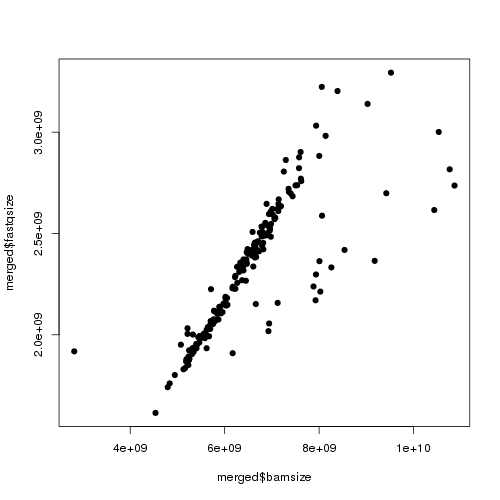
Each point is one sample, and I’m plotting each sample’s BAM size against the size of one of its two gzipped FASTQ files. Basically, I find that one FASTQ is usually about 36-41% the size of the resulting BAM (I’m using paired end reads and comparing to only one FASTQ, so this implies that the two FASTQs are ~80% the size of the BAM, thus that the alignment information adds about 1/.8-1 = 25% to the compressed size of the data). You see a very tight correlation between BAM size and FASTQ size (streak in the middle). Then on the left you see one smaple where the BAM is much smaller than it could be – this makes me suspect that job failed in some mysterious way, so I flag it as a “badbam” and re-run it later. There are also usually a few BAMs that are larger than they should be (dots towards the right). I haven’t figured out why that occurs.

Note that when I first aligned the 192 samples I just submitted them as 192 jobs. My priority in my institution’s LSF queue isn’t high enough for there to be any advantage for me in parallelizing that process even further. But now that I have (in the example above) just one sample that needs to be re-aligned, I can benefit from splitting it up to run in an hour or so instead of a few days.

This I do “manually” since it’s one sample, pasting the paths into these commands:

bsub.py medium 08:00 "gunzip -c /data/HD/dataset/mouse_ki_allele_series_rnaseq/20130424-H22819.FASTQs/514_Liver_Q111_HET_M_L8.LB9_1.clipped.fastq.gz | split -d -a 3 -l 1000000 - tmp1.list"
bsub.py medium 08:00 "gunzip -c /data/HD/dataset/mouse_ki_allele_series_rnaseq/20130424-H22819.FASTQs/514_Liver_Q111_HET_M_L8.LB9_2.clipped.fastq.gz | split -d -a 3 -l 1000000 - tmp2.list"
ls # check how many files this created. in this case, split files are numbered 000 through 177
for i in {000..177}
do
    bsub.py short 00:50 "gsnap --format=sam --read-group-id=514 --read-group-library=LB9 --read-group-platform=illumina -N 1 -m 10 -d grcm3873ki tmp1.list$i tmp2.list$i | samtools view -Sbh - > tmp.list$i.bam"
done
bsub.py medium 23:00 "samtools merge 514_Liver_Q111_HET_M_L8.LB9.bam `ls tmp.list*.bam | tr '\n' ' '`"

Basically I gunzip -c the FASTQs, i.e. decompress while keeping the original, and pipe that to split the data into n one million line files (-l 1000000) with 3 digit identifiers (-a 3) and the prefix tmp1.list for the first end of the pair and tmp2.list for the second end of the pair. Then I check how many files this created, loop through them all and submit a separate Gsnap job for each. Then I samtools merge the bams back together. tr to eliminate newlines in the ls output is from this awesome StackOverflow answer.

Or alternately if you had more than one sample fail, you can grep -f the badbam list against the fastq.12col file to re-run only those jobs.

Once I’m confident that all the BAMs have aligned properly, I sort and index. You can cat fastq.12col | awk '{print $3".bam"}' to get the list of BAMs, or to save trouble you can just iterate over the list of BAMs as I do here. Again, I copy everything to a temporary directory and then back again.

mkdir srtd
for bamfile in *.bam
do
  bsub -q medium -W 20:00 -m general "workdir=/my/working/dir; tmpdir=\$(mktemp -d); trap 'rm -rfv \$tmpdir' EXIT;  cp $workdir/$bamfile \$tmpdir; samtools sort \$tmpdir/$bamfile \$tmpdir/$bamfile.srtd; samtools index \$tmpdir/$bamfile.srtd.bam; mv \$tmpdir/$bamfile.srtd.bam $workdir/srtd; mv \$tmpdir/$bamfile.srtd.bam.bai $workdir/srtd; rm \$tmpdir/$bamfile"
done

This gives me sorted, indexed BAMs in a folder srtd/ with names that end in .bam.srtd.bam.

step 5. expression levels

Once I’ve got sorted indexed BAMs I usually want to get some sort of gene expression levels. There’s a healthy debate to be had about the right measure of gene expression to use depending on what your research question is. See my post on counts vs. FPKMs, and in particular Richard Smith‘s comment. For many purposes, transcripts per million (TPM) may be the best metric [Li 2010]. TPM can be calculated using RSEM. I’m currently learning how to use RSEM and if I get a good pipeline up and running with that tool I’ll add that as a new post in the future. In the meantime, this post will cover how to run Cufflinks and get FPKM values for each transcript in your GTF file.

Here’s how I did it:

mkdir cufflinks
mkdir cufflinks/1
cat fastq.12col | awk '{print "cufflinks -o cufflinks/1/"$3" -G /data/HD/public/GRCm38.73/Mus_musculus.GRCm38.73.gtf gsnap/1/srtd/"$3".bam.srtd.bam"}' > cufflinks.bash
less cufflinks.bash # examine bash script
cat cufflinks.bash | awk '{print "bsub.py medium 23:00 \""$0"\""}' | bash

When I first started learning RNA-seq it surprised me that Cufflinks runs separately on each sample. It seemed that this process was missing the gene expression analogue of joint calling of genetic variants, as for instance in exome sequencing. I now realize that if you’re doing differential gene expression you often run Cuffdiff after Cufflinks, and Cuffdiff sort of serves this role of comparing all the samples to each other.

Incidentally, if you want to go rogue and analyze gene expression levels on your own, without Cuffdiff (and I make no statement as to how advisable this is), here’s a quick bit of bash to combine all the Cufflinks output files into one relational file with a SAMPLEID column.

mkdir ../combined
# prep header rows
cat 847_Liver_Q92_HET_F_L5/isoforms.fpkm_tracking | head -1 | awk '{print "SAMPLENAME\t"$0}' > ../combined/all.isoforms.fpkm_tracking
cat 847_Liver_Q92_HET_F_L5/genes.fpkm_tracking    | head -1 | awk '{print "SAMPLENAME\t"$0}' > ../combined/all.genes.fpkm_tracking
# combine files
for subdir in *
do
    # combine isoforms data into one file, adding a column for sample name
    cat $subdir/isoforms.fpkm_tracking | tail -n +2 | awk -v subdir=$subdir '{print subdir"\t"$0}' >> ../combined/all.isoforms.fpkm_tracking
    # combine gene symbol data into one file, adding a column for sample name
    cat $subdir/genes.fpkm_tracking | tail -n +2 | awk -v subdir=$subdir '{print subdir"\t"$0}' >> ../combined/all.genes.fpkm_tracking
done

Which took under a half hour. Once I have gene expression levels (be they FPKMs or otherwise) I next move into some version of my gene expression QC pipeline, which I won’t repeat here.

step 6. coverage plotting

In my particular project, we have a couple of different research questions, some of which revolve around gene expression (hence Cufflinks or some other tool, above) and others of which will require some custom scripting to look at coverage around particular splice sites and polyadenylation sites. Therefore among other things I want to calculate read depth for a region of interest, which I do here using BEDtools.

First I need to create a BED file listing the genomic regions I’m interested in. In this case, I want mouse huntingtin (called Hdh or Htt depending on who you ask) as well as the knock-in construct that I added to my reference genome.

cat > htt.bed
5	34761743	34912534
Hdh_Q_ki_construct	0	799
^D

And then I use BEDtools coverageBed:

bamfile=gsnap/1/srtd/test.bam.srtd.bam # first try on my small "test" file
coverageBed -abam $bamfile -b htt.bed -split -d > $bamfile.htt.cov 
# assuming the above test worked ok, then:
for bamfile in *.bam
do
    bsub -m general -q medium -W 02:00 "cd /my/working/dir/; coverageBed -abam $bamfile -b htt.bed -split -d > $bamfile.htt.cov"
done

Each job takes < 1 hour (I set the wall limit to 2h just to be safe.) Note the use of two options here. -d gets base pair depth at every single base of the features of interest. -split is essential for RNA-seq: when a read is split over two exons, -split prevents it from contributing to coverage calculations for the spanned intron.

The coverageBed -d output gives me five columns, which I’ll refer to as (in order): contig, start, stop, relindex, and depth. Each row just describes the depth at one particular base located at contig:(start+relindex), so all the information here can be expressed in just 3 columns (contig, start+relindex, depth). Moreover, I’ve just created 192 coverage files for 192 samples, all in exactly the same format, so I can just combine these into a matrix and save a lot of space. Here’s how:

mkdir ../combined
mkdir ../1col
# create a file to hold just the contig and base columns
cat > ../combined/locations.txt 
contig base
^D
cat test.bam.srtd.bam.htt.cov | awk '{print $1" "$2+$4}' >> ../combined/locations.txt
# now create a 1-column version of all the coverage files
for covfile in *
do
  echo $covfile | awk -F"." '{print $1}' > ../1col/$covfile.1col # add a header row with the sample name (and some extraneous stuff)
  cat $covfile | awk '{print $5}' >> ../1col/$covfile.1col # add just the depth column ($5)
done
# paste them all together
paste ../combined/locations.txt ../1col/* > ../combined/allsamples.cov # paste all the samples together into a matrix
# remove clutterfiles
rm ../1col/*

You can then pull allsamples.cov into R and plot depth vs. base pair position for any sample (or combination of samples).

conclusion

I’m not including any downstream analysis here because I wanted to keep this general. This was just a quick overview of how I’ve been aligning reads and getting coverage and expression levels. I hope it’s useful and I welcome any feedback.