Genetics 25: 'Mapping the genetic basis of complex phenotypes'
These are my notes from lecture 25 of Harvard’s Genetics 201 course, delivered by Steve McCarroll on November 21, 2014.
Today’s topic is how to map complex (polygenic) traits and diseases, or what is a genome-wide association study?
How to study polygenic traits
Doing a GWAS is analogous to mapping monogenic traits/disorders except that you are working with unrelated individuals, which means that there have been far more recombination events since their most recent common ancestor, and the haplotype blocks are much shorter. You need thousands of such unrelated individuals in order to have any power.
Linkage disequilibrium
Suppose you genotype two SNPs, SNP1 and SNP3 and you find that the genotypes are as follows:
| SNP1 | SNP3 | count |
|---|---|---|
| AA | CC | 49 |
| AG | CT | 42 |
| GG | TT | 9 |
In this example, none of the other possible combinations (for instance, SNP1 = AG and SNP3 = CC) are seen at all. This indicates perfect linkage disequilibrium between the two SNPs. An individual’s genotype at SNP3 can be predicted perfectly based on their genotype at SNP1. This means there are two haplotypes in the population being studied:
| haplotype | SNP1 | SNP3 |
|---|---|---|
| haplotype 1 | A | C |
| haplotype 2 | G | T |
Now suppose that there is an additional SNP, SNP2, between these two, and that the haplotypes in the population including SNP2 are as follows:
| haplotype | SNP1 | SNP2 | SNP3 |
|---|---|---|---|
| haplotype 1 | A | A | C |
| haplotype 2.1 | G | A | T |
| haplotype 2.2 | G | G | T |
Now you can see that the G allele of SNP2 is seen only on a “haplotype 2” background. SNP2 is therefore also in linkage disequilibrium with SNP1 and SNP3, even though it cannot be predicted perfectly.
Note that linkage refers to the connection of alleles within families, which occurs on a scale of tens of megabases, whereas linkage disequilibrium refers to the analogous phenomenon in unrelated individuals, usually on a scale of tens of kilobases.
One measure of linkage disequilibrium is r2. It is calculated as follows. The input data are a list of individuals (rows) and their alt allele count at various SNPs (columns), for instance:
IID SNP1 SNP2
1   2    2
2   1    1
3   0    1
4   2    2
5   1    1
6   1    1
7   0    0
Then r is the Pearson’s correlation coefficient of the SNP1 and SNP2 columns. r2 is 1.0 for SNPs in perfect LD, and 0.0 for unlinked SNPs. For the example above, r2 for SNP1 and SNP2 is between 0 and 1.
The first effort to comprehensively map linkage across the human genome was HapMap, which used genotyping of ~6M SNPs [International HapMap Consortium 2003]. 1000 Genomes has also mapped linkage, using sequencing [Abecasis 2012].
Genome-wide association studies (GWAS)
Linkage disequilibrium is important because it allows genome-wide association studies (GWAS). In GWAS, typically 300,000 to 1 million SNPs are genotyped, and an additional ~5M are imputed based on those. The fact that SNPs are in LD with one another means that you don’t need to genotype every SNP in the genome in order to figure out what genomic locus is involved in a trait. If a common SNP affects a trait, then even if you do not genotype that SNP, you will probably genotype one that is in LD with it (a “marker” SNP) and that marker will be correlated with your trait of interest.
A typical GWAS involves the following steps:
- Collect genomic DNA from thousands of cases and thousands of controls
- Genotype 300K to 1M SNPs on an array (cost: ~$50 per sample)
- Impute 5-10M SNPs
- Test each SNP for association with a phenotype
Consider the follwing data for one SNP and a dichotomous phenotype:
| genotype | cases | controls |
|---|---|---|
| AA | 2 | 4 |
| AG | 16 | 22 |
| GG | 32 | 24 |
In an additive model, instead of considering these three genotypes, we can just take the count of each allele:
| allele | count in cases | count in controls |
|---|---|---|
| A | 20 | 30 |
| G | 80 | 70 |
Nominally, the A allele seems to be more common in cases. To test whether this is significant, we can use a Chi squared test. In the absence of true phenotypic association, the expected number of A alleles is 25 in each group, and the expected number of G alleles is 75 in each group. The Chi squared statistic for deviation from this null hypothesis is given by:
χ2 = Σ (observed - expected)2/expected
χ2 = (20-25)2/25 + (30-25)2/25 + (70-75)2/75 + (80-75)2/75
χ2 = 52/25 + 52/25 + 52/75 + 52/75
χ2 = 2.67
This value can then be looked up in a table to get a p value. Steve McCarroll endorses this Chi-square calculator. You can do the whole calculation in R as follows:
ctable = matrix(c(20,80,30,70),nrow=2)
chisq.test(ctable)
With the result:
    Pearson's Chi-squared test with Yates' continuity correction

data:  ctable
X-squared = 2.16, df = 1, p-value = 0.1416
So in this case, the difference in allele frequency is not even nominally significant (p = .14).
In practice, you’d do this all in PLINK or maybe PLINK2.
An important fact to note about GWAS is that the associated allele is always seen in cases and in controls. These alleles contribute to a trait or to disease risk, but they are not Mendelian - they do not wholly determine the trait or disease.
Now let’s return to the above example but suppose that all the numbers are 100 times larger, such that the result is actually significant:
ctable = matrix(c(2000,8000,3000,7000),nrow=2)
chisq.test(ctable)
    Pearson's Chi-squared test with Yates' continuity correction

data:  ctable
X-squared = 266.1336, df = 1, p-value < 2.2e-16
Great - now the p value is less than 5e-8, which is the typical threshold for genome-wide significance (this concept is introduced below).
For the sake of argument, let’s suppose that this association also holds up after controlling for population stratification, so we believe the SNP is truly associated with the trait.
Now that we have a significant association, we might want to know the effect size of this SNP. Effect size can be measured by odds ratio. For this table:
| allele | count in controls | count in cases |
|---|---|---|
| A | 3000 | 2000 |
| G | 7000 | 8000 |
The odds ratio is given by:
8000 * 3000 / (2000 * 7000) ≈ 1.7
For a more detailed tutorial on what an odds ratio is, how to calculate it and when it applies, please see the difference between odds ratio and risk ratio.
Controlling for multiple statistical tests
A nominal p value gives the proportion of times that, if the null hypothesis were true, you would see a result at least this extreme just by chance. In statistical tests where the null hypothesis is true, the p values should be uniformly distributed from 0 to 1. Therefore if you perform 20 statistical tests, on expectation one test will give a p value less than .05. Similarly if you perform 1 million statistical tests, on expectation one test will give a p value less than 1e-6.
To determine which SNPs are truly associated with a trait, we need some measure of how often we would get a result at least this extreme even given how many tests we’ve performed. One simple way to do this is using Bonferroni correction, which is simply dividing by the number of independent statistical tests we’ve performed. The human genome contains roughly 1 million haplotype blocks and therefore, even if you test 6 million SNPs for association with a trait, you’ve only done about 1 million independent statistical tests. Therefore, it is generally held that the threshold for genome-wide significance is 5e-8, which is a nominal threshold of p = .05, Bonferroni-corrected by dividing by 1 million.
A typical way of displaying results from a GWAS is to plot the -log10(p value) for each SNP on the y axis, against the SNP’s chromosomal position on the x axis. This is called a Manhattan plot. Here is an example from this useful post:
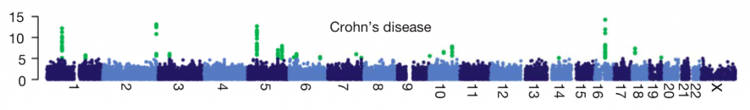
A linkage peak in a Manhattan plot will usually contain many different associated SNPs (if it doesn’t, that’s a bad sign). These different SNPs do not represent separate associations, just a bunch of SNPs that are all in LD with each other and with a causal SNP that affects the trait.
Lessons from GWAS
- Many traits are highly polygenic. GWAS have revealed that many traits and diseases have a very large number of contributing loci. So far we have seen >200 loci for height, >500 for body mass index, >100 for schizophrenia and ~200 for Crohn’s disease.
- Effect sizes of common variants are small. The linked loci from GWAS tend to have odds ratios in the range of 1.05 to 1.30, indicating that common variants tagged by GWAS hits each contribute only a little bit to the overall phenotype. Therefore, GWAS hits are not very useful for “personalized risk prediction”, even though they are useful for discovering genes and pathways.
- Most, but not all, associations are near genes. The genes near GWAS SNPs include some expected genes (for example, genes already known to be implicated in Mendelian forms of the trait/disease) as well as many novel genes, which tend to cluster into pathways. There are also a few interesting exceptions, where a trait-associated SNP is in a “gene desert”, very far from any gene.
- Most associations point to regulatory DNA, not to coding variants. For most phenotypes, about 80% of the GWAS associations involve haplotypes that are entirely confined to non-coding sequence, such as introns or upstream of genes.
- Associated SNPs have a strong tendency to be located in open chromatin. Many are near histone marks that correspond to enhancers. Many also correspond to expression quantitative trait loci (eQTLs) for the tissue relevant to the phenotype of interest.
It is believed that these lessons from GWAS tell us something generalizable about complex trait variation in populatons. It is now thought that much of the variation in these traits is due to quantitative dials on expression levels of different genes in different cell types, rather than to variants affecting the encoded proteins themselves.
The road forward
Now that we have GWAS results, where do we go from here? In schizophrenia there are now >100 associated loci, yet they collectively explain only ~15% of the estimated heritability of schizophrenia. There are various theories of where the “missing heritability” lies - depending on whom you ask, it might lie in genetic interactions (epistasis), larger effects in the truly causal variants than in the tagging SNPs, or in rare variants of large effect.

About Eric Vallabh Minikel
Eric Vallabh Minikel is on a lifelong quest to prevent prion disease. He is a scientist based at the Broad Institute of MIT and Harvard.