Circular dichroism on recombinant PrP
This month we completed our first recombinant PrP prep here at the Broad Institute. As one in a series of next steps to check whether we had produced properly folded protein, we performed circular dichroism (CD) on it. I was totally new to this technique, and this post will share what I learned from the expert at Broad who generously trained us. For what it’s worth, everything here has been said in other, more thorough, tutorials on CD out there on the web (such as this or this).
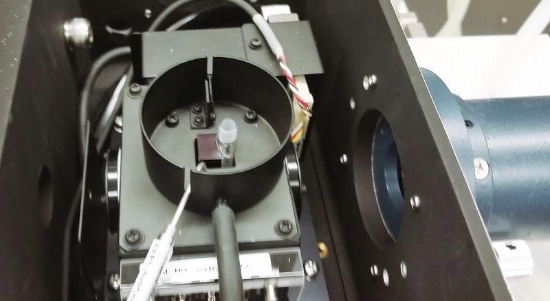
Circular dichroism is a technique that measures differential absorption of circularly polarized light in order to gain low-resolution information about the secondary structure of a protein. This is the best explanation I’ve read of the underlying physics. The term “CD” seems to be used both to refer to the technique and to the thing being measured; the device that does it (pictured at top) can be called a CD spectrometer. In our case, we wanted to do CD to check whether our recombinant PrP had turned out largely alpha helical, as it is supposed to.
Fortuitously, the concentration of protein in our prep, only 3.4 μM or 0.08 mg/mL, despite being too low for RT-QuIC, is perfect for CD. Also fortuitously, our dialysis buffer had come out at just the right pH with just sodium phosphate buffers (which are invisible to CD), so we never adjusted the pH with HCl (chloride ions can interfere with CD).
CD uses the mid-to-far ultraviolet, 190 to 260 nm, so it is performed in these tiny rectangular vials called cuvettes or cells, which are made of quartz, which is UV invisible. You can’t touch the flat front or back, because smears from your fingers will cause false signals. Always grip it by the sides. We used a cuvette with a 2 mm path length, referring to the thickness of the protein solution that the laser beam will pass through. Shorter path length means a skinnier tube, which means you use less volume of protein (in our case, only ~300 μL), although if you don’t heat your protein, CD is non-consumptive anyway — you can just pipette the protein back out when you’re done and use it again for something else. There also exist thicker cuvettes with a 10 mm path length, which is useful if you are heating your protein and you want to put the thermometer right in the cuvette, but apparently you can get a pretty good temperature reading with the thermometer adjacent to the cuvette anyway. The ultraviolet lamp has to operate in pure nitrogen, so start the flow of N2 several minutes before you are ready to use the machine to purge any air that is in it.
Before you add any protein, just take a spectrum on a completely blank cuvette. If the last person to use it didn’t clean it properly, you’ll see a signal of protein stuck to the quartz. To check this, just a quick, cursory reading is fine. Thus we set the “accumulations” (number of readings that will be averaged together) to just 1. And we set the scan speed to 100 nm/min. That means that the whole spectrum, from 260 nm down to 190 nm, will be taken in under a minute. Here are the settings we used:
![]()
And sure enough, the first cuvette we scanned was dirty: you could see a substantial deviation from zero at some wavelengths, indicating it was picking up secondary structure of some residual protein stuck to the cuvette (blue curve below). We tried a second cuvette and it was clean — there was no signal, we were told, beyond just the inherent noise of CD (green curve below).
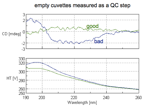
A note on how to read these plots: the top half is the CD spectrum. The x axis is the wavelength of light being absorbed, and the y axis is circular dichroism in millidegrees (mdeg - more on that unit later). The bottom half is dynode voltage, labeled as high tension (HT). These two references both agree that for any wavelengths where HT rises above 600 V, that means that your sample is “saturated” (absorbance is too high) and the signal is not meaningful, so you can disregard any information at those wavelengths.
Next we took the good cuvette and filled it with water as a blank. Actually, if we’d had the foresight to do so, we would have saved some dialysis buffer as a blank (this is now in my checklist at the bottom of this post). To read the blank, we dropped the scan speed to 50 nm/min, and used 5 accumulations, so the whole scan took several minutes. Note the scale on the y axis - all we see here is a really small amount of noise, comparable to the empty cuvette:
![]()
To get the water out of the cuvette, we just used one of those really long, thin pipette tips that people use for Western blots. Then we added in 300 μL of protein and scanned it again. To get a final plot of our data, we applied two transformations. First, we subtracted the baseline. Second, we converted the CD (y axis) from millidegrees to molar ellipticity so that it would be comparable between proteins. This conversion is per the following formula (explained here):
\[\Delta\varepsilon = \frac{\Delta A}{C \times I}\]Where:
- Δε = CD in molar ellipticity
- ΔA = CD in millidegrees
- C = molar concentration of peptide bonds
- I = path length in mm
You’re dividing millidegrees by molarity and millimeters, so the units of molar ellipticity end up being deg·M-1·m-1. In our case, our protein concentration was 3.4e-6 M, and it is 208 amino acids, so it has N-1 = 207 peptide bonds, so C = 3.4e-6 × 207 = 7e-4, and our path length was 2 mm. Thus, our readings which were on the order of 10-20 millidegrees ended up being on the order of 10,000 - 20,000 deg·M-1·m-1. Now that we have our spectrum expresed in molar ellipticity, we can compare, say, HuPrP23-230 to HuPrP90-230. If you stay in units of mdeg you can only compare a protein to other samples of the exact same protein.
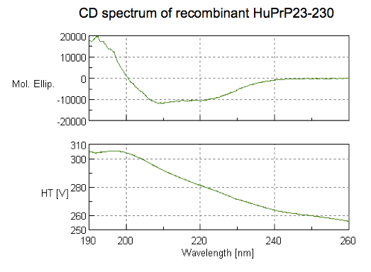
With all that said, here is what our spectrum looked like:
How to interpret this? Different secondary structures have different characteristic CD spectra, so alpha helix looks different from beta sheet looks different from a disordered polypeptide [Greenfield 2006]. The standard absorbance spectra for these secondary structures come from decades-old experiments [Greenfield & Fasman 1969] on poly-L-lysine (K~800), which can be induced to adopt pure alpha helix, beta sheet, or random coil conformations depending on the pH and heat treatment it is subjected to. Here are the standard spectra for polylysine in its various conformations (data, code):
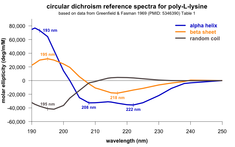
In the plot I’ve labeled a few wavelengths that are considered reference points. For instance, alpha helices give peak negative absorbance at 208 and 222 nm, and positive absorbance at 193 nm. Our spectrum fits this pattern, consistent with substantial alpha helical content — exactly what we were hoping for. The data are also consistent with some contribution from beta sheet, which is negative at 218 nm and positive at 195 nm. In contrast, if we had an unfolded protein, we’d expect negative absorbance at 195 nm and almost zero absorbance above about 210nm. The overall conclusion, then, is that we have a protein, and it is folded.
There are many different pieces of software out there that will take your protein’s spectrum and try to deconvolute it as a linear combination of these three polylysine spectra. These may also take into account the fact that individual aromatic residues (F, W, & Y) contribute to absorbance as well. But we were cautioned against doing this, as it might lead us to overinterpret our data. Apparently CD spectra are pretty good at telling you if your protein has some (say, >10%) alpha helical content, but aren’t very well-powered to discriminate between, say, 30% vs. 70% alpha helix. Indeed, looking back at this post I remembered that deconvolution of early CD spectra on PrPSc (the infectious, misfolded form of PrP) had suggested that it contained 20% alpha helix [Safar 1993], which no one believes nowadays [Requena & Wille 2014].
By now we’ve confirmed that we have a folded protein. The other question that CD allows us to ask is at what temperature that fold will be lost, or in other words, the melting point of the protein. One way to do this is by heating your sample and taking a full CD spectrum at every temperature. But it is much quicker to just measure at a couple of characteristic wavelengths, so we set up the machine to only take readings at 208 and 222 nm — the two negative bands for alpha helices — while heating the sample from 20°C to 90°C. Here’s the curve we obtained:
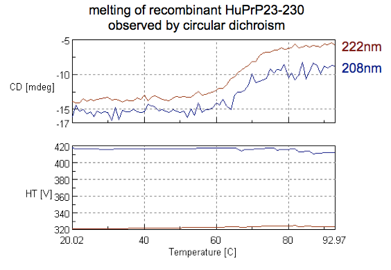
Just eyeballing it, you can see that both wavelengths follow the same pattern, with an decrease in the magnitude of negative absorbance indicative of secondary structure being lost from 60°C to 70°C. The melting point or Tm is apparently taken to be the median on this curve, which is hard to say exactly because it’s pretty noisy, but appears to be around 65°C. That sounds about right. I couldn’t find any references for full-length human PrP, but reports indicate that recombinant HuPrP 121-231 melts at 71°C [Calzolai & Zahn 2003] and that 91-231 melts at 66.1°C [Nicoll 2010], so we’re probably in the right ballpark.
To review, then, the protein we made seems to be folded, and it has approximately the melting point we expect for PrP. All good signs.
After finishing with CD, the final step is to clean the cuvettes, which involves filling them with 5M nitric acid for a few hours or overnight. The nitric acid doesn’t damage the quartz, so they can even be left over the weekend if need be. Only the inside needs to be cleaned with nitric acid; if anything gets on the outside, a kimwipe is probably enough to wipe it off.
Finally, here’s a short draft checklist for the next time we do CD:
- Start N2 flowing into the machine.
- Take a reading on the empty cuvette.
- Take a reading on the blank buffer.
- Ignore data at HT >600 V.
- After reading, subtract the blank and convert to molar ellipticity.
- Turn off N2.
- Clean cuvette with nitric acid.

About Eric Vallabh Minikel
Eric Vallabh Minikel is on a lifelong quest to prevent prion disease. He is a scientist based at the Broad Institute of MIT and Harvard.