NMR fragment screening
what is fragment screening?
Over the past few years I’ve done a lot of thinking about high-throughput screening as a starting point for drug discovery in prion disease — see for instance this and this. Over the past few months I have started learning about an approach, fragment-based screening, which is considered largely orthogonal to conventional high-throughput screening, and which has on numerous occasions succeeded in identifying probes for targets against which conventional screening campaigns had previously failed [Hajduk & Greer 2007]. This blog post will contain some of the most basic things I’ve learned about this method, both by reading about it and by talking to Mike Mesleh, the Broad Institute’s resident expert on biomolecular NMR. I’m writing this post largely to solidify my own understanding; if you’re just looking for a good introduction to the topic of fragment screening, you can find lots of content on the web written by people who are actually experts in this technique — see for instance these reviews [Hajduk & Greer 2007, Chessari & Woodhead 2009, Erlanson 2012], and the blog Practical Fragments.
So what’s the difference between conventional and fragment screening? In a word, size. Fragment screening means screening smaller molecules than is usually the case for high-throughput screening. How small? Here’s a comparison of the molecular weight distribution in 1.05 million ChemBridge compounds (a conventional HTS library) versus 4,397 ACB Blocks compounds (a fragment library):
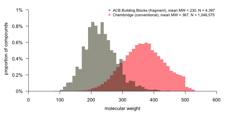
Code to produce this plot.
why fragment screening?
But why would particularly small molecules be of particular interest?
One argument concerns ligand efficiency [Hajduk & Greer 2007]. Ultimately, the drug you’re trying to develop probably needs to be larger than just a fragment, because additional binding surface gives you more affinity and more specificity, which you need. But with increased size come extra pharmacokinetic liabilities, so you want to make sure your molecule consists of nothing more than the bare minimum structure needed to hit the target. In a conventional high throughput campaign, you’re starting from larger molecules that probably have some unnecessary chaff that you will need fight to to whittle away. Fragments can only bind if they have higher ligand efficiency, meaning more of the fragment is involved in the binding, so you’re starting with the minimum, and then you add onto it only where the additions improve potency.
Another argument that has been made is one of chemical diversity [Hajduk & Greer 2007]. For the past decade, a group led by Jean-Louis Reymond at University of Berne has set about calculating the number of possible molecules of various sizes [Fink 2005, Reymond 2015]. Trivially, the number of possible molecules of 1 atom is just the number of different elements you’re willing to consider — say, C, N, O, S, and maybe F and some other halogens (usually hydrogens are implicit and so are not considered). The number of possible molecules of N atoms is a function of how many unique graphs of that many vertices you can draw, and then how many different ways you can permute the allowable atoms into it, and then how many of those structures actually abide by the rules of chemical bonds in our universe. The number of possible molecules containing N atoms turns out to be exponential in N — roughly 10⅔N, looking at Figure 2A of [Ruddigkeit 2012]. One interpretation of this is that the smaller size of molecules you focus on, the larger a fraction of possible chemical space, in that size range, you can hope to cover. If you consider molecules of up to 17 atoms, there are about 1011 possible molecules, and their mean molecular weight is around 240 Da [Ruddigkeit 2012] — similar to the ACB Blocks fragment library above. So if you screened those 4,397 ACB Blocks compounds, you’d have screened roughly 1 out of every 107.5 possible molecules of that size. The Reymond group has not yet enumerated all the molecules of 27 atoms, but at least according to the trend so far, there would probably be something like 10⅔×27 = 1018 of them, and at an average of about 14 Da per atom they’d have a mean molecular weight comparable to that of the ChemBridge library, and so even if you screened all 1 million ChemBridge compounds, you’d still only be looking at only 1 in every 1012 possible compounds of that size. Based on this argument, fragment screening allows you to access a greater (though still small) fraction of all possible chemical diversity, and thus should give you better odds of hitting a difficult target.
But so far, all I’ve made are theoretical arguments. Probably, the real reason why fragment-based screening has become popular is because several success stories have demonstrated that it works, meaning it can be used to design potent ligands, often for difficult targets. Many such successes are discussed in the reviews I mentioned up top [Hajduk & Greer 2007, Chessari & Woodhead 2009, Erlanson 2012], and I’ll call out a few here.
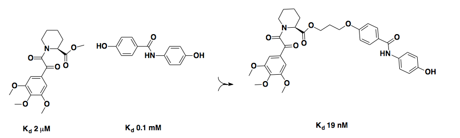
This first example, above, is from the original paper putting forth NMR-based fragment screening as a method [Shuker 1996]. They were seeking new ligands for FKBP12, which had just been described as the target of FK506 a few years earlier [Liu 1991]. In a screen of 10,000 fragments, the two shown at left were found to bind FKBP12 at adjacent sites with micromolar affinity, and linking them together yielded a 19 nM affinity ligand. Because the primary screen gave binding site information, it was easy to progress from that screen to linking the two adjacent fragments, so this method was described as “SAR by NMR”. Although there were certainly other people who had screened low molecular weight libraries before, this paper demonstrated the power of doing so with NMR, and so many scientists credit Shuker’s work as marking the dawn of fragment-based screening [Chessari & Woodhead 2009, Lepre 2011].
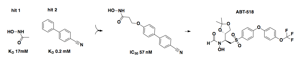
The above example comes from Abbott Pharmaceuticals and is adapted from [Hajduk 1997, Wada 2002] via [Hajduk & Greer 2007]. It is a beautiful example of how two low (millimolar) affinity fragments (left) that bound at adjacent sites were linked to form an amazingly potent ligand (center) — a nanomolar probe of matrix metalloproteinase 3 (MMP3). The company later shifted its focus to a different matrix metalloproteinase, and another analog (ABT-518, right) optimized for that target eventually made it to a Phase I clinical trial [Hajduk & Greer 2007].
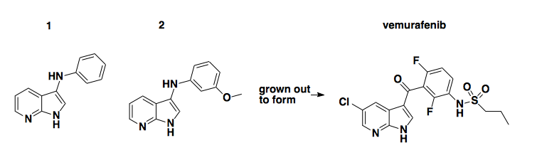
This example chronicles the discovery of vemurafenib by Plexxikon Inc [Tsai & Lee 2008]. They did a fragment-based screen of 20,000 compounds and found a series of 7-azaindoles which inhibited kinases (albeit at concentrations ≥200μM) by binding to kinase active sites. They don’t report what exactly the original hits looked like, but through iterative optimization they arrived at compound 1 (~100μM IC50), then 2, then PLX4720 (right; almost identical to PLX4032, which is vemurafenib), which inhibits BRAF V600E kinase activity with an EC50 of 13 nM, which is >10-fold selectivity over wild-type BRAF and >100-fold selectivity over most other kinases. Vemurafenib is pretty legendary: it went from discovery [Tsai & Lee 2008] to FDA approval in only 3 years. It was the first molecule developed from fragment-based screening ever to become an approved drug.
how does fragment screening work?
Those are some examples of what you can achieve with fragment-based screening. But how do fragment-based screens actually work? It turns out that the choice of very small molecules has a lot of profound consequences for the practical implementation of the screen. The “ligand efficiency” concept discussed above means that fragments can have strong affinity for their size, but that’s still a very weak affinity in absolute terms. As shown in the examples above, the fragment hits that serve as starting points for optimization often have affinity (Kd) in the millimolar range. To find such hits, you need a screen that is very sensitive, or one that you can run at very high concentration (say, hundreds of micromolar), or both. In fact, fragment screening is sometimes referred to as “high concentration screening”. The high concentration, in turn, has a lot of consequences. Compound aggregation is already a big source of false positives in conventional screens at 10μM [McGovern 2002], so if unchecked it would be an enormous problem in fragment screens. To prevent this, only the most soluble fragments can be screened.
In some cases, biochemical screens can be amenable to these very high concentrations. For instance, in the vemurafenib example, the primary screen was actually for fragments that inhibited kinase activity [Tsai & Lee 2008]. But ultimately, some of the unique advantages of fragment based screening come from the ability to intelligently grow and link fragments based on your knowledge of where and how they are binding. So at some point, you need information on the binding site and binding orientation. In the vemurafenib example, this was obtained at the secondary screen stage via X-ray crystallography. I was amazed to learn that there are some relatively high-throughput methods for X-ray crystallography [Kumar 2005, Jhoti 2007], and some people have actually managed to use crystallography as a primary screen [Nienaber 2000, Chessari & Woodhead 2009]. Another creative approach is to screen covalently reactive fragments and then perform mass spec to figure out which cysteines (whether endogenous, or ones you’ve engineered into sites you’d like to bind) the fragments reacted with [Erlanson 2000]. But the most popular fragment screening approach seems to be NMR. NMR gives binding site information, can be performed with compound concentrations in the hundreds of micromolar, and can actually detect a fragment’s interaction with a ligand even at concentrations far below its Kd.
NMR fragment screening in practice
To get a sense of how these screens work in practice, I read one very thorough guide to how to implement NMR fragment screens [Lepre 2011]. From my conversations with Mike Mesleh, it sounds like Lepre’s guidance accords pretty well with how NMR fragment screens are typically performed here at the Broad Institute. Here’s what a typical screen might look like.
Before beginning any sort of screen, it is important to get comfortable producing your recombinant protein, and extensively QC it. For starters, you may want to run a gel to confirm the identity of your protein, and perform circular dichroism and/or 1H NMR on it to confirm that it is folded. Then you’ll want to produce 15N-labeled protein, which you can produce by growing your bacteria in minimal media with any 15N-labeled media supplement, like this one, as the sole nitrogen source. With the labeled protein you can perform heteronuclear single quantum coherence (HSQC) spectroscopy. This is a 2-dimensional NMR technique where you get one axis for the 15N nuclei and one for the 1H nuclei, which gives higher-resolution structural information than you can get from 1H NMR alone. You can do the HSQC at a few different temperatures so that you’ll know if your protein is prone to undergo any conformational switching. And because a fragment screen will take a few days to run to completion, you will want to leave your protein sitting out for a few days and then check that it is still stable. You’ll also want to use differential scanning calorimetry, or a similar technology, to obtain a melting curve for your protein, and test any available positive controls for their ability to influence that melting curve.
As a primary screen, one can perform “ligand-observed” NMR. That is, you load the small molecule ligand(s) and the protein into an NMR tube, and you run NMR to observe the ligand, while subtracting out the protein’s signal. So you are looking for chemical shifts in the ligand that would indicate it is binding to something. This requires that in advance of screening, you collect a reference spectrum on each ligand by itself so that you know what you’re looking at. Typically you can use 1H NMR for ligand-observed techniques, although there are also fragment libraries where all the fragments contain fluorine, and you can do 19F NMR — see this Practical Fragments post. In a ligand-observed screen, you use unlabeled protein, which is easier to produce than 15N-labeled protein. The protein doesn’t need to be in any special buffer, just PBS at a neutral pH, plus you’ll end up with a final concentration of about 1% DMSO after adding the compounds. In this environment, any disulfide bonds will be formed rather than reduced. You can screen the ligands in batches of, say, 8 compounds per tube, which saves you NMR tubes, protein, and time. The ligands are usually present at 200 μM each, in about 1% DMSO final, and remember, because NMR can detect interactions at below the Kd, this concentration even allows you to detect millimolar binders. Indeed, rather than missing weak binders, you actually risk missing ligands whose affinity is too strong, because at nanomolar binding, the on/off rate is too low for a fragment to exhibit detectable chemical shifts. The protein is usually present at 10 μM, so you have a 20:1 ligand:protein stoichiometry. A primary screen will usually be on the order of a few thousand compounds, though some people will do low tens of thousands. For a primary screen of, say, 2,000 compounds with 8 compounds per tube and 180 μL volume per tube, you end up needing about 45 mL of protein at 10 μM. So for PrP, for instance, with a molecular weight of 22 kDa, this ends up being a total of about 10 mg of recombinant protein. After the pooled primary screen, the next step is to re-test any hits as singletons, meaning with only 1 small molecule per tube instead of 8, which might cost you another few mg of protein.
Any compounds that pass this test will then move on to “protein-observed” NMR using 15N-labeled protein. 15N media supplements are a bit pricey, and protein yields also tend to be a bit lower than with unlabeled protein — two reasons why it’s often preferred to do a ligand-observed screen as primary, and then only run the protein-observed screen as a secondary. Here, you need higher a protein concentration, say 50 to 100 μM, and you have to screen the compounds in singlicate — otherwise, since you’re not observing them, you wouldn’t know which was binding. But you’ll probably be testing only, say, 100 compounds at this point, so at 180 μL volume per tube and 100 μM concentration, that still only costs you about 4 mg of protein. The compounds are still screened at 200 μM. The protein-observed technique will provide orthogonal conformation of binding events, and will also allow you to observe the binding site of each compound.
People make every effort to remove bad-behaving compounds from fragment libraries, but still, there are always a lot of sources of false positives, particularly since the compound concentrations used are so high. One obvious source of false positives, as in conventional HTS, is compound aggregation. Another thing is a lot of compounds will have metal impurities left over from synthesis, and if the compound is at 200 μM, then even a 0.5% contaminant is still present at 1 μM and can easily give a false positive. Furthermore, in pooled screening, compounds can interact or react with each other; obviously, the groups of 8 compounds are chosen to minimize this possibility, but it’s still a concern. And again, since the concentrations are so high, acidic or basic compounds can actually have a substantial impact on the pH, which can in turn affect the protein’s behavior and give a false positive. Many more pitfalls are discussed in [Lepre 2011, Davis & Erlanson 2013].
For all these reasons, there are a lot of follow-up assays you’ll want to do after screening. The quickest way to rule out a lot of aggregators is to re-test the compounds in NMR with a little bit of non-ionic detergent such as Triton or Tween. You can also perform dynamic light scattering (DLS) to check if your compounds are aggregating. Surface plasmon resonance (SPR) is a confirmatory assay which will also allow you to measure the Kd of your compounds, so that you can prioritize some of the stronger binders. Differential scanning calorimetry (DSC) is another valuable confirmatory assay, which lets you detect changes in your protein’s melting temperature upon compound binding. Remember that at the screening stage, you’re just looking for hits that are real, not for potent binders at this point, so even a fraction of a degree of thermal shift in DSC should be enough to reassure you that a hit is real.
After you’ve done all these confirmatory assays, hopefully you’ve whittled your initial hit list down to a list of ligands that you are confident are really binding. Next you can start strategizing about which hits are good starting points for medicinal chemistry efforts to obtain more potent ligands. Although your protein-observed NMR will have given you some information about which residues are affected by ligand binding, it is not trivial to figure out exactly where and how each ligand binds. So a good next step is to use some structural biology software to model the compounds’ interactions with the protein and try to figure out in exactly what orientation they are binding. This will allow you to focus on pairs or groups of ligands that bind at adjacent sites and, as in the examples above, might be suitable for linking together. And before hauling off and starting any new chemical synthesis, the lowest-hanging fruit is usually to search through commercial catalogs and find any compounds that are close analogs of your hits, so that you can test those and start to get some preliminary structure-activity relationships. This approach is colloquially known as “analog by catalog”.
After all those steps, it’s time to move into serious chemistry efforts to try to grow or link your compounds into something with stronger affinity and drug-like potential. Here, of course, you have the same challenges as in any drug discovery effort, trying to simultaneously optimize your compound on several dimensions, including potency, pharmacokinetics, and low toxicity. But with luck, at least you’ve got a lead or two to start from, which you might not have found through conventional screening.

About Eric Vallabh Minikel
Eric Vallabh Minikel is on a lifelong quest to prevent prion disease. He is a scientist based at the Broad Institute of MIT and Harvard.