Isothermal titration calorimetry
Last week I learned how to perform isothermal titration calorimetry (ITC). Here’s what I learned.
principles
ITC is a useful tool for studying direct interactions between two molecules in solution — for example, a protein and a small molecule ligand. It can not only inform on whether a binding event occurs, but also provide data on the thermodynamic parameters of the interaction.
In ITC, one of the two molecules is stored in a chamber called the sample cell and the other is injected into that cell from a syringe. For sake of example, we’ll say the protein is in the sample cell and the small molecule is in the syringe, though these roles can be reversed. Next to the sample cell, a reference cell contains the exact same buffer but with neither protein nor small molecule in it. As the small molecule is injected into the sample cell, it and the protein may bind, releasing heat. The reference cell and sample cell have very precise thermometers, and tiny heaters working to keep them at the same temperature. By measuring the difference in how much energy has to go into the two heaters to maintain the same temperature (isothermal) during the injection, the instrument can determine the amount of heat energy released by the binding event (calorimetry). By adding the small molecule into the sample cell over a series of small injections (titration), the instrument can gather data sufficient to determine the thermodynamic parameters of binding.
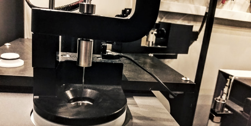
Above: closeup of the ITC syringe engaging the cell.
GE offers this helpful tutorial describing both the principles of ITC and the use of this machine in particular. Here’s a diagram I adapted from their tutorial depicting how the data typically look and what you can infer from them:
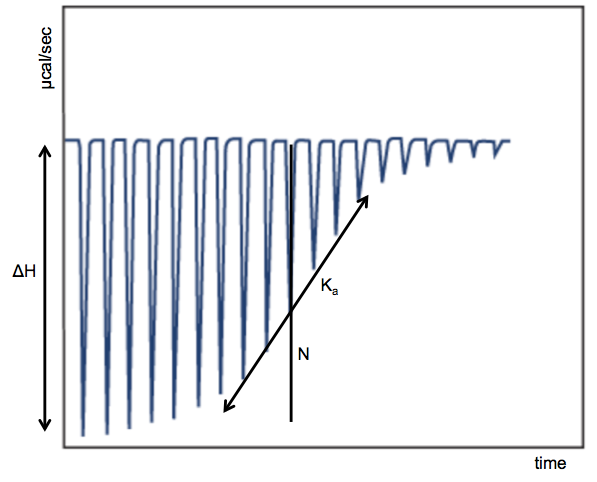
The x axis is time, the y axis is rate of heat release (μcal/sec), and each spike represents one injection. For the first few injections, the small molecule is less abundant, so it all immediately gets bound by protein, releasing the maximum amount of heat that it is capable of releasing, per mole of small molecule. Thus, the magnitude of the early spikes tells you the ΔH, or enthalpy of binding. As you inject more small molecule, you begin to saturate the protein, which gives you a sigmoid shape, culminating in a flat curve at far right when the protein is all already ligand-bound. The slope of the middle of the sigmoid curve tells you the association constant, or Ka. The more commonly referred-to dissociation constant is just its inverse: Kd = 1/Ka. The midpoint of the sigmoid curve occurs at N, the molar ratio of binding. If each copy of the protein binds one copy of the ligand, then the midpoint of the curve should occur when the two molecules are equimolar, N = 1.
As explained helpfully in these OCW notes, the Gibbs free energy of binding is related to the association (or dissociation) constant. ΔGassociation = RTlnKa or ΔGdissociation = RTlnKd. And we also know that binding is driven by enthalpy and entropy: ΔG = ΔH - TΔS. So having observed Kd and ΔH, it is possible to also infer ΔS — the entropy of binding.
When I sat down to work through the math, I realized just how sensitive an instrument the ITC is. In our case (as will be explained more below) we performed 20 injections of 2 μL each of a 1 mM solution of our small molecule. That means that each injection contained 2e-6 L at 1e-3 mol/L = 2e-9 mol = 2 nmol of small molecule. The enthalpy was determined to be on the order of -4 kcal/mol in the first full injection (before the protein was saturated with ligand) which means that the energy released in the binding event of that injection was 4e3 cal/mol × 2e-9 mol = 8e-6 cal = 8 microcalories. Remember that a calorie raises 1 g = 1 mL of water by 1°K. So 8 microcalories would only raise the temperature of (say) a 100 μL ITC cell by 8e-5 °K, and even if all 20 injections released this much heat, that would still be only a .0016 °K temperature increase.
in practice
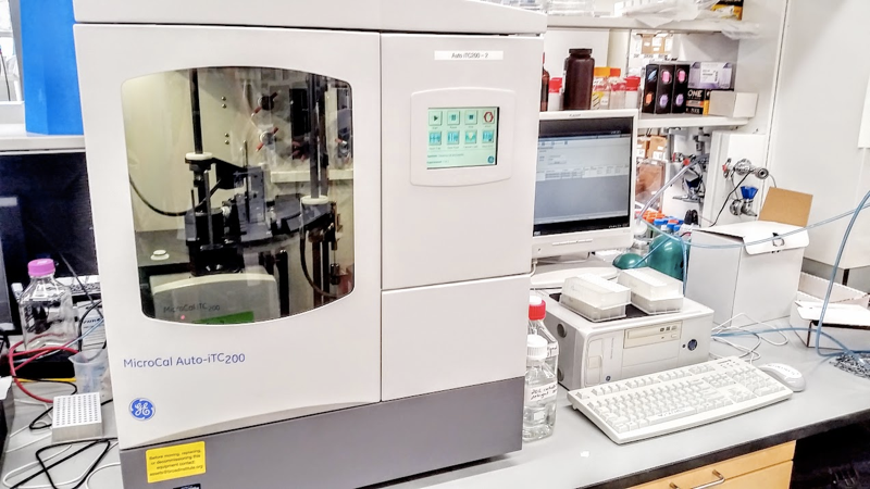
Broad has a GE MicroCal™ AUTO-iTC200. Experiments are set up in deep 96-well plates. Each ITC experiment takes up three wells of the plate — one each for protein (for the sample cell), compound (for the syringe), and buffer-only (for the reference cell) — and takes on the order of 2 hours, depending on exactly what settings you choose. Most of that time is spent on cleaning and liquid handling; the actual experiment is more like 40 minutes. Usually, it is a good idea to also run a control where you have only buffer in both the sample and reference cell, and inject compound into it — this can help you keep from getting tricked by artifacts where just diluting the compound releases energy. Thus, a typical setup might involve 6 wells and 4 hours total:
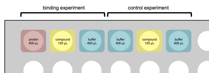
Remember that the 1st, 2nd, and 3rd wells (and their respective volume requirements) just correspond to sample cell, syringe, and reference cell. Unlike what’s depicted above, you can choose to put 125 μL protein in the syringe and 400 μL compound in the sample cell.
The ideal ITC experiment, as depicted in the example plot further up in this post, gives you a full sigmoid curve. Depending on your Kd, you can tweak the protein concentration, compound concentration, and number and size of injections to try to achieve this curve. If you don’t know the Kd (maybe that’s why you’re doing ITC in the first place), a good starting point is 25 μM protein in the sample cell and maybe 800 μM or 1 mM compound in the syringe. The AUTO-iTC200 does injections at a rate of 0.5 μL/sec, and a typical protocol might be 20 injections of 4 seconds (2 μL) each, with a 180 second break between injections to allow the cells to reach equilibrium.
ITC is incredibly sensitive to buffer conditions. It is essential that the buffer for the protein, the compound, and buffer-only conditons be the dialysis buffer from dialyzing the protein. Simply measuring out the same ingredients and calling it the same buffer is not good enough. Adding DMSO after the fact to match the DMSO concentration in the compound is usually a necessary evil, but one still needs to interpret data with caution. According to that GE tutorial I mentioned earlier, even a difference of 2% DMSO vs. 1.95% DMSO can result in a weak but detectable heat release upon each injection. Also, buffers that release heat when they ionize are problematic. Luckily, phosphate and HEPES (the only two buffers we have ever used with PrP here) are both acceptable. Since PrP is extracellular, we leave our recombinant PrP oxidized, but if you need a reducing agent, apparently TCEP is permissible but DTT is not.
So when setting up the experiment, remember to dilute your protein and compound in the dialysis buffer that you’ll use as the buffer-only reference, and to have the same concentration of DMSO (if applicable) in every cell. For instance, if you have a 100 mM compound stock in 100% DMSO, you could mix 2 μL of your stock with another 3 μL of DMSO (order of addition matters for solubility) and then add 245 μL of dialysis buffer, for a final 250 μL of 800 μM compound in 2% DMSO — enough for both your binding experiment (125 μL) and control experiment (125 μL). In order to match your other solutions exactly, dilute your protein to 25 μM in dialysis buffer and then add 2% DMSO, and add 2% DMSO to the reference buffer-only condition as well. You can prep all these solutions in Eppendorf tubes before transferring them to the plate.
a pilot experiment
In order to learn ITC, I did a simple pilot experiment to see if I could replicate something that has been reported in the literature.
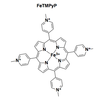
Four independent research groups have reported that an iron porphyrin referred to as FeTMPyP (above) binds to PrPC and exhibits antiprion properties, with low micromolar potency [Caughey 1998, Nicoll 2010, Massignan 2016, Gupta 2016]. One of these groups reported an ITC experiment for FeTMPyP binding to N-terminally truncated recombinant human PrP [Nicoll 2010, Figure 1].
We ordered FeTMPyP from Cayman Chemical earlier this year and made a 100 mM stock in water. (In our experience it actually dissolves more readily in water than in DMSO). For protein I used recombinant HuPrP90-231 produced Rocky Mountain-style and dialyzed against 20% CSHL PBS at pH 7.4. (This was our 13th batch of recombinant PrP, and we had a yield of 55 mg from 1L of bacterial culture — we’ve come a long way since last December!) The protein had been frozen at -80°C at 112.5 μM (spec’ed on the NanoDrop).
Here’s what my prep looked like:
- 1 mM compound: dilute 3 μL FeTMPyP (100 mM in water) in 297 μL of the protein’s dialysis buffer
- 25 μM protein: dilute 111 μL of 112.5 μM protein in 384 μL of dialysis buffer and 5 μL of water (to match the water the FeTMPyP is dissolved in — yes, I’m being that rigorous about buffer matching). Note that recombinant HuPrP90-231 weighs in at about 16 kDa, so this experiment costs about 0.5 mg of protein.
- buffer-only: combine 1386 μL of dialysis buffer with 14 μL of water (again, to match the solvent of the FeTMPyP)
I added 400 μL of protein to well A1, 125 μL of compound to A2 and A5, and 400 μL buffer to A3, A4, and A6.
The instrument’s operating software is fiddly and not always intuitive, so here are a few points:
- Your ultimate goal is to get the Experiments tab to reflect the actual physical layout of your plate. The Sample Groups tab is simply a tool to help you populate the table on the Experiments tab. The Automation Method determines the number of wells per experiment. We use Plates Prerinse Syringe Clean, which gives 3-well experiments as I’ve described here.
- In the “Data File” column of the Experiments tab, be sure to specify filenames that are unique over the first 10 characters. The instrument’s operating software will let you save with any length of filename with any length constant prefix, but when you later open your data in the instrument’s analysis software (Origin Data Analysis), it will only load datasets by the first 10 characters of their filename, and it is literally unable to hold two datasets of the same 10-character name open at the same time. If you accidentally already gave your files long repetitive names, you’re not out of luck, though: you can navigate to the raw .itc text files stored on disk and rename them. The filename itself is the only record of the experiment’s name.
- The number and size of injections and other parameters are stored in an “ITC Method” on the Instrument Setup tab. The list of ITC Methods displayed here is simply a list of .inj files found in a particular directory (on our instrument, C:\ITC200\Setup). You can use Save As to create a new ITC Method, but save it in that same directory — if you save it in, say, a subdirectory with your name, it will not appear in the ITC Methods list.
- After you fill out the Experiments tab, click “Validate” and the software will predict how much water, methanol, detergent, and waste capacity will be needed. Empty or refill bottles as appropriate. Only once this is done should you click Play.
We ran the experiment under the standard protocol of 20 injections of 4 seconds (2 μL) each, with 180 seconds between injections, and it was done within 4 hours.
I haven’t had a chance to really work on understanding the format of these .itc raw text files yet but in case anyone wants to dig in, here they are:
- FeTMPyP2HuPrP902301.itc - binding experiment
- FeTMPyP2buffer1.itc - buffer-only control
In principle, here’s what the analysis stage consists of. The text files describe the energy released as a function of time in each injection. You integrate to obtain the total energy release per injection. You fit a sigmoid curve to these points, and the parameters of that fitted curve tell you ΔH (enthalpy), Ka (association constant), and N (molar ratio).
I haven’t dug into the raw data myself, instead relying so far on what is apparently the standard pipeline for analyzing these data in the Origin Data Analysis software that comes with the machine. This pipeline is a bit tricky, so here’s a step-by-step. Go to File > New Project… and then on the background (not the menu bar) click “Read data…” and select the binding and control experiments, in that order, Add File(s) and click OK. The software will take several seconds to do a bunch of analyses in the background. You can click through the windows (Window menu) and see the raw ITC data, the tables, and the processed data. The raw curves in our case looked like this:
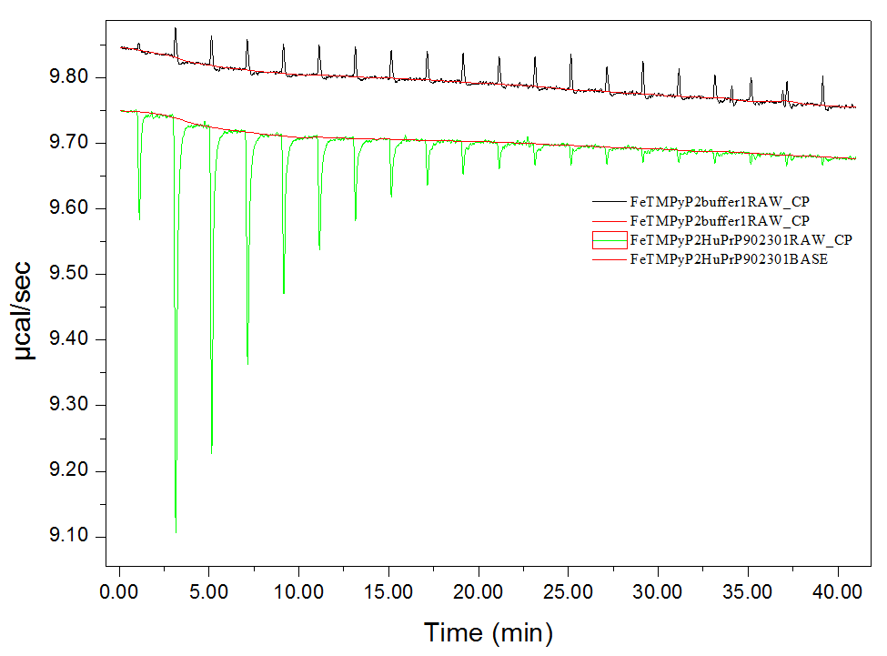
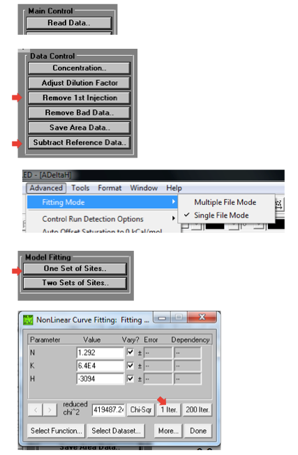
Green is the binding experiment, where the negative spikes represent heat released at each injection, and black is control, where the positive spikes (of much smaller magnitude) apparently represent some minor endothermic property of diluting the compound into buffer. The Window > ADeltaH tab will show you the processed data, with points representing the area under the curve of each injection spike. Click on “Subtract Reference Data…” to subtract the control points from the binding experiment points, and “Remove 1st Injection…” because the ITC does a little test injection of only 0.4 μL first before it starts the “real” injections, and this outlier shouldn’t be used in curve fitting. Then go to Advanced > Fitting Mode > Single File Mode. Click on “One Set of Sites” under Model Fitting on the background buttons, which will take you to a Nonlinear Curve Fitting window, where you can click “1 Iter” a few times until the numbers stop changing. This is just fitting the sigmoid curve to the processed data.
I found it very easy to get confused about which buttons to click in the software, because there are many similar-looking options. Here is a quick guide:
At the end of all that, you’ll have a curve with a fitted line and parameters. To make a nice 2-panel plot with the subtracted data as well as the model and fit, go to Analysis > Final Figure. If you want the legend with the fitted thermodynamic parameters to display, you have to copy and paste it over from the ADeltaH window where it was born. You may also want to fiddle with axis display increments as the defaults aren’t always legible. Here’s what my data looked like:
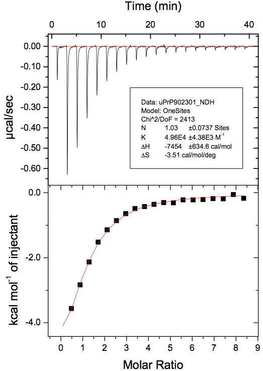
Note that the first 0.4μL test injection is still represented in the raw data (top panel) but has not been used in the curve fitting (bottom panel).
Here’s some interpretation of these data:
- ΔH = -7.5 kcal/mol. That GE tutorial says that -5 kcal/mol is “average”, and it’s hard to say what they mean by that, but at least I infer we’re at least on the order of magnitude that is usually seen with ITC.
- N = 1.03. Nominally, this means that the molar ratio is ~1, so FeTMPyP has a single binding site on PrP and binds in a 1:1 stoichiometry. However, because we don’t have a full sigmoid curve (it gets flat on the far right but not on the far left), the N is considered uninterpretable. To be confident that 1 is the correct answer, we would need to re-run the experiment and get more points further left on the x axis, at a molar ratio of <1.
- Ka = 4.96e4 M-1. We take the inverse (1/Ka) find that Kd = 2.0-5 M. So the Kd of FeTMPyP for PrP in this experiment is 20 μM.
- ΔS = -3.5 cal/mol/°K. The negative value indicates that entropy is actually fighting this binding event, which is being driven entirely-and-then-some by the negative enthalpy.
interpretation
I am excited that this experiment worked — ITC was easy to learn, quick to set up, and should be a good way to validate any screening hits that appear to bind PrP. That said, like any technique it does have some caveats, particularly the need for binding to be enthalpically driven, the dependence on buffer conditions, and the difficulty of getting a nice full sigmoid curve for certain Kd values.
The dissociation constant (Kd) that we obtained for FeTMPyP binding PrP is 20μM. That’s slightly higher than has been reported previously, though this could simply be a matter of the experimental details. In [Nicoll 2010] they did several ITC experiments, varying the PrP construct (Hu91-231 or Hu119-231), the experimental design (protein in cell and compound in syringe or vice versa), and the buffer conditions (low or physiological NaCl), and obtained several answers ranging from 3 μM to 11 μM. Our entropy value for FeTMPyP, -3.5 cal/mol/°K, is also of a slightly a larger magnitude than reported — [Nicoll 2010] reported values of -0.5 and -1.5. If you figure ΔG = ΔH - TΔS, and ΔH = -7.5 kcal/mol, T = 298°K (room temperature), and ΔS = -3.5 cal/mol/°K, then overall ΔG = -6.4, with the enthalpy driving it and the entropy slightly fighting it.
In spite of there being so many different groups that have reported FeTMPyP binding PrP, and in spite of our own data here validating a release of heat energy when FeTMPyP is titrated into PrP, I still can’t shake a certain skepticism about whether FeTMPyP is a “real” binder in the sense of binding specifically and at a defined binding site on PrP’s surface. Porphyrins are known to derive some of their bioactivities through aggregation (try a Google Scholar search for “porphyrin stacking”) and certain other antiprion porphyrins have been seen to aggregate [Nicoll 2010]. FeTMPyP apparently binds bovine serum albumin with a Kd of ~10 μM [Massignan 2016], similar to its affinity for PrP. On top of all that, FeTMPyP is also fluorescent, chelating, and NMR-quenching (because iron is ferromagnetic). It’s a perfect storm of potentially assay-busting properties. Yet it undeniably does possess some genuine bioactivity, and here in ITC and in many other assays [Massignan 2016] it behaves beautifully, and makes for a handy positive control.

About Eric Vallabh Minikel
Eric Vallabh Minikel is on a lifelong quest to prevent prion disease. He is a scientist based at the Broad Institute of MIT and Harvard.