What can we learn about PRNP from gnomAD v4?
The long-awaited v4 release of gnomAD contains DNA sequence data from 807,192 humans. We have learned new things about prion disease with each previous release, and now our sample size is 6 times larger. In this post, I dig into the variants in PRNP to see what we can learn about mutational saturation, genetic prion disease prevalence, and the functional impact of truncating variants.
mutational saturation
In 2020, I posted this plot illustrating how many out of the possible single nucleotide variants in PRNP had been observed in gnomAD V2. I downloaded the gnomAD v4 variant CSV file for PRNP in order to update this†.
†Remarkably, the only two updates required were an offset to convert from GRCh37 to GRCh38, and a formatting change for converting the chromosomal position to a string. Kudos to the gnomAD production team for not breaking backward compatibility in 4 years of software development!
Here is the new plot (link takes you to a high-resolution PDF):

Since it has been 4 years, let’s remind ourselves what we are looking at above. Every box here represents one possible single nucleotide variant in PRNP’s coding sequence. The coding sequence is 762 base pairs long, and every base pair can convert to the 3 other possible base pairs, for instance, an A could become C, G, or T, so there are 762 × 3 = 2,286 boxes. Each box is sized proportional to the expected mutation rate giving rise to that variant. The sizes differ because for instance, a C is 10x more likely to become a T (a transition) than to become an A (a transversion), and it’s yet another 10x more likely to become a T if the following base is G (a CpG transition) — this has all been worked out empirically by studying de novo mutations in humans [Samocha 2014]; if you want a mechanistic reason why it is so, don’t ask me, ask a chemist. They’ll say something about deamination. The boxes are shaded according to presence/absence in gnomAD. Present = opaque, absent = translucent. And they are colored and ordered by functional impact. Gray = synonymous, orange = missense, maroon = predicted loss-of-function.
At a glance, what you see is that a lot of the plot is filled in. To be exact, 52.0% of the plot is opaque, meaning PRNP is halfway to mutational saturation. That’s in the DNA of 807,162 humans, and these things are nonlinear, so it by no means guarantees that we’ll hit full saturation in 1,614,324 humans, but it is a huge change from 2020 when we had 141,456 people. To see just how much more filled-in the plot is, here’s the side-by-side. Below is the 2020 version, mouseover shows 2024:

2020 v2 version by default, 2024 v4 version on mouseover. Mouseover code from here.
Here’s a breakdown by mutational class (CpG, Ti = transition, Tv = transversion) and functional impact:
| mutational class | functional impact | observed/possible | percent observed |
|---|---|---|---|
| CpG | missense | 29/29 | 100% |
| CpG | ptv | 1/1 | 100% |
| CpG | synonymous | 16/16 | 100% |
| Ti | missense | 149/463 | 32% |
| Ti | ptv | 11/33 | 33% |
| Ti | synonymous | 83/220 | 38% |
| Tv | missense | 131/1203 | 11% |
| Tv | ptv | 5/59 | 8% |
| Tv | synonymous | 29/262 | 11% |
Percent of all possible variants observed in PRNP in gnomAD v4, by mutational class and functional impact.
That’s right, we are now 100% saturated in CpG variants — every possible CpG mutation in PRNP has now been observed in a living human. Other than that, we’re still a ways off — only ⅓ saturated for non-CpG transitions and 10% saturated for transversions. That’s why I say it’s nonlinear and we still won’t be at saturation when we hit 1.6 million people.
Nonetheless, one implication of how far we are along the road to saturation is that we have to be careful about dynamic range for things like constraint. CpGs are so saturated now that it may no longer be possible to see constraint by looking at them — not for an adult-onset disease like prion disease. (For genes where mutations cause embryonic lethality or severe pediatric disease, CpG constraint should still be valid). For starters, 3 really bad CpG transitions — P102L, D178N, E200K — are all present in gnomAD, even though we know they are highly penetrant causes of genetic prion disease [Minikel 2016, Minikel 2019]. As for whether this is surprising, or consistent with disease prevalence, see the next section.
Whereas, in the transition (Ti) statistics, there is a whiff that we observe just slightly fewer of the missense transitions than the synonymous transitions (32% vs. 38%). It is non-significant (OR = 0.78, P = 0.17 by Fisher test, contingency table below), so there may or may not really be missense constraint here. But certainly, if you wanted to know whether there was missense constraint, CpGs are no longer where you would go looking for it.
| synonymous | missense | |
|---|---|---|
| absent from gnomAD v4 | 137 | 314 |
| present in gnomAD v4 | 83 | 149 |
Contingency table of PRNP non-CpG transitions by functional class in gnomAD v4.
A final point to note is that the denominator is very different between mutation classes. There are twice as many possible transversions as non-CpG transitions, and about 15 times as many non-CpG transitions as there are CpG transitions. So although we’re 52.0% saturated in mutational probability space, we’re only 20% saturated in terms of unique mutations.
If constraint is no longer interpretable for CpG variants, are pathogenic and benign variants really indistinguishable? From first principles, when we think about constraint, and ask whether a variant is present at all, we are simply scraping the Poisson or negative binomial distribution from the rightmost edge of a normal distribution. As the sample size gets larger and we slide our viewing window leftward, into rarer territory, that normal distribution comes into full view. As that happens, we might expect there should start to be some relationship between pathogenicity and allele frequency. It won’t be perfect: benign variants can have high frequency because of drift, or they can happen to not have gotten swept up in any drift, and still be very low frequency. But constraint wasn’t perfect either — pathogenic variants could happen to appear once, and benign variants could happen to appear zero times — you always had to average across a large enough list of variants to get anything meaningful.
How, then, does the frequency distribution look for our PRNP CpG variants? Below, I plot the gnomad AC (on a log axis, since all are >0 now!) against the prior mutation probability from [Samocha 2014]:
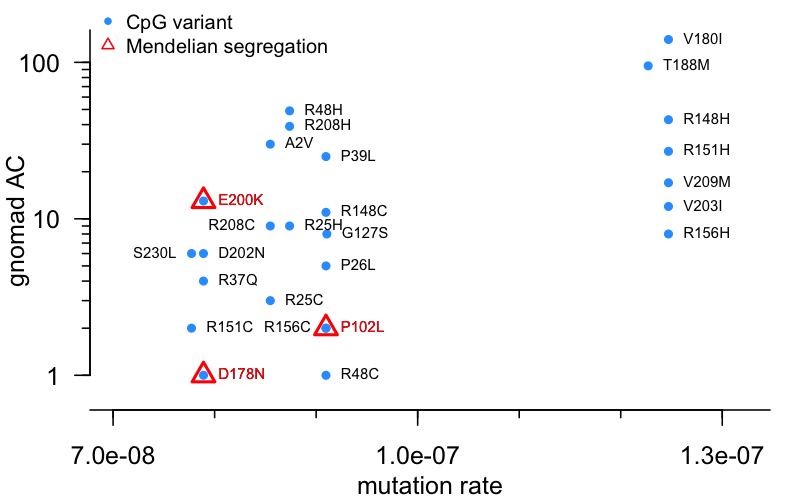
Remember that, while CpG variants occur much more frequently than non-CpG transitions, there is still some variabiilty among CpGs. Several PRNP variants, spread out at the right side of the plot, arise from a C→T transition within an ACG context, which is the most mutable of all. All of those variants have an AC of at least 8 — to me, this provides some hint that even among CpG variants, mutation rate matters. Of all possible CpG variants here, while several do or may affect prion disease risk a little bit, only 3 have strong evidence for high penetrance in the form of Mendelian segregation — these are highlighted in red triangles. 2 of the 3 are very low frequency, 1 or 2 alleles in gnomAD, less than most variants of a similar mutation rate. Just E200K is an outlier, with an AC of 13. Let’s unpack that more in the next section.
prevalence of genetic prion disease
As prion disease is a notifiable disease, its frequency is fairly well studied. I have unpacked what’s known in two previous blog posts: prion disease is not one in a million and how many patients do we have. Long story short, genetic prion disease is the cause of roughly 1 in 50,000 deaths. You can arrive at very roughly this same figure by a variety of methods: multiplying the annual incidence of prion disease by the proportion of cases that are genetic by the average human lifespan; reviewing death certificates and dividing prion disease deaths by total deaths, then multiplying by proportion genetic; or by capture-recapture (described in that latter post). While this figure is certainly a rough estimate, it’s not going to be off by logs. Remember, this 1 in 50,000 is the proportion of deaths caused by genetic prion disease, or you could think of it as the genetic prevalence — the proportion of people at birth who have a mutation that would cause them to later develop genetic prion disease (until/unless we succeed in our quest).
We can ask whether the prevalence of highly penetrant mutations in gnomAD is consistent with this estimate. If we mash up gnomAD data with the list from [Goldman & Vallabh 2022] Table S1 (also kept up-to-date here) of which PRNP variants have reported Mendelian segregation with disease in families — evidence for high penetrance — we get the following:
| variant | mutation class | gnomAD AC |
|---|---|---|
| P102L | CpG | 2 |
| D178N | CpG | 1 |
| E196K | Ti | 1 |
| E200K | CpG | 13 |
That’s a total of 17 individuals with high penetrance variants, out of 807,162 individuals. That’s 1 in 47,480. At first glance, you say wow, that’s almost spot-on with our estimate of genetic prevalence. On second glance, it’s actually just a bit higher than expected, once you consider the age distribution in gnomAD (I re-plotted this combining the exomes and genomes):
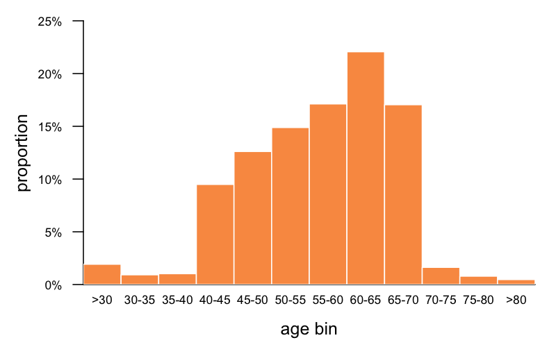
Age information is only available for 63% of gnomAD, and what exactly it means varies by cohort (age of ascertainment, age of last followup, age blood sample taken, etc.) but at a minimum, it means someone was alive at the given age. What you can see is that gnomAD skews older than the population at large, and certainly a lot older than zero, which is the age we’re talking about when we speak of genetic prevalence at birth being 1 in 50,000. Based on this age distribution and what we know about age of onset in genetic prion disease, we can estimate by what proportion we would expect high penetrance variants to be depleted in gnomAD. At a glance, we can see that just 41% of gnomAD individuals are under 55, which is around the median onset for P102L and D178N (estimated at 56 and 53 respectively in [Minikel 2019] Table 1); 58% are under 60, which is around the median onset for E200K (62 in [Minikel 2019] Table 1, or estimated at 64 in [Minikel 2014]). So intuitively, we might guess that only 41% or 58% of carriers of these respective mutations would live long enough to have the possibility to appear in gnomAD.
To formalize this intuition, we should speak not in terms of medians but of the full distribution. I take the life tables for each mutation (such as E200K) and, for every age, multiply the probability of survival at that age (Pt, column pt) by the proportion of gnomAD individuals that are that age. Summing across all the ages should give us the proportion of carriers of this mutation, from birth, that would still be alive in the gnomAD age distribution. (Note that I’ll focus here on the 3 most common causal variants in genetic prion disease; for E196K we have too little data).
| variant | proportion alive in gnomAD age distribution |
|---|---|
| P102L | 40% |
| D178N | 37% |
| E200K | 61% |
We can further mash this up with the proportion of high-penetrance genetic prion disease cases caused by each variant — 49% E200K, 19% P102L, 17% D178N. (Since we don’t have full survival curves for most of the other variants, we’ll consider the 85% of cases caused by these 3 variants to be our “universe”). Summing the product of these figures by the proportion alive in the above table and normalizing to the total fraction of cases caused by these variants (85%), we come to a final estimate of 51%. This means that 51% of high-risk genetic prion disease variant carriers from birth will survive long enough to appear in the gnomAD age distribution. Therefore, when we see a prevalence of 1 in 47,480 in gnomAD, that would imply a prevalence of 1 in 24,215 from birth. High-risk mutations are about twice as common in gnomAD v4 as we expected.
There are several possible explanations, and more than one may contribute. Here I’ll focus this discussion on E200K, since that variant contributes 13 of the 17 alleles:
- Underdiagnosis. The number of prion disease cases diagnosed is rising faster than the population is growing and aging [Maddox 2020], suggesting that prion surveillance systems haven’t yet reached saturation and we may still be underdiagnosing by a bit. Underdiagnosis is probably most severe for mutations with “atypical” presentations, and somewhat less so for E200K, which usually has a “classical” presentation much more like sporadic CJD. However, another potential way in which underdiagnosis could contribute is if a somewhat higher percentage of cases are genetic than we’ve assumed. In our 2016 study, only a subset of prion disease cases had undergone PRNP sequencing, such that cases known to have a genetic variant were 12% of all cases but 18% of sequenced cases. It turns out it’s not actually hard for these factors combined to explain the frequency we see in gnomAD. We assumed that prion disease kills 1 in 6,000 people and 12% of cases are genetic, for a genetic prevalence at birth of 1 in 50,000. If the reality were 1 in 5,000 and 18%, that would give us 1 in 27,778 at birth — very close to the 1 in 24,215 at birth implied by the gnomAD v4 data.
- Sampling variance. While 17 in 807,162 corresponds to a point estimate of 1 in 47,480 in this age distribution, or 1 in 24,215 at birth, the Wilson 95% confidence interval would extend to 1 in 76,043, or 1 in 38,782 at birth. That gets us a good chunk of the way towards our expectation of 1 in 50,000 at birth. Consistent with sampling variance playing a role, in 2016 when we looked at 531,575 people in 23andMe, we found ≤5 alleles of P102L, A117V, D178N, and E200K combined.
- Founder populations. There are E200K founder effects in Slovakia, Sicily, and Israel (among Libyan Jews) — and that’s just the few we know about. If any of these populations is over-represented in gnomAD that could explain it. The 13 E200K individuals in gnomAD are Finnish (N=1), Admixed American (N=2), and non-Finnish European (N=10); no further detail on ancestry is publicly available.
- Penetrance. A couple of papers have claimed E200K penetrance to be as low as 60% [D’Alessandro 1998, Mitrova & Belay 2002], but both in small sample sizes, with no raw data presented and no description at all of the methods used. This has always made it hard to credit these estimates as opposed to the larger, more thorough studies that have arrived at a ~90% figure [Chapman 1994, Spudich 1995, Minikel 2014]. That being said, 90% is only a rough estimate, and there are ascertainment biases in all these studies. If the truth is lower, that could be one contributor.
- Phenotypic enrichment. A risk with any gnomAD analysis is that if your disease phenotype looks like one of the phenotypes on which gnomAD cohorts were ascertained, then causal variants look more common than they are. That could be a factor here, since there are Alzheimer and ALS cohorts in gnomAD v4, but it’s probably not a major factor, since again, most E200K cases have a classical rapid dementia phenotype that is relatively more easily recognied as prion disease and would only rarely be mistaken for AD or FTD.
Considering all these potential factors, it is actually pretty easy to reconcile the gnomAD data with our expectations.
For truncating variants, on the other hand, it’s another story.
protein-truncating variants (PTVs)
ExAC v1 and gnomAD v2 both told a relatively straightforward story about protein-truncating variants (PTVs) — nonsense and frameshift — in PRNP [Minikel 2016, Minikel 2020]. N-terminal truncating variants (codon 131 and earlier), which are likely to be cause loss of function by removing most of the protein altogether, are found in healthy controls and are unconstrained — we see no evidence of natural selection against them in a heterozygous state. C-terminal truncating variants (codon 145 and later), which leave most of PrP intact but remove the GPI anchor, causing a change in localization, cause a pathogenic gain of function and are found in dementia cases. We had long known that such C-terminal PTVs were found in prion disease, and the one such variant in gnomAD v2 turned out to belong to an individual ascertained on a diagnosis of Alzheimer’s, which we suspect was a misdiagnosis.
Before we go further, an essential piece of background is that whereas “typical” prion disease is a rapidly progressive dementia fatal within months, C-terminal truncating variants in PRNP give rise to a really different “atypical” phenotype [Mead & Reilly 2015]. Patients may present first with chronic diarrhea due to secreted PrP amyloid deposition in the gut and are often misdiagnosed with inflammatory bowel disease (IBD). Eventually this progresses to peripheral neuropathy due to deposition in peripheral nerves, and after decades it becomes a slowly progressing dementia easily misdiagnosed as Alzheimer’s or FTD.
In gnomAD v4, as expected for a 6-fold increase in sample size, there are a lot of new PTVs. But surprisingly, the picture may also be more complicated, because a number of the PTVs that we see are C-terminal. Including filtered variants, gnomAD v4 reports a total of 33 unique PTVs in PRNP. I manually curated them all and removed 4:
- W7X is a real variant and might be a real LoF, but there exists a possibility of rescue by residue M8 as an alternate start codon
- H69MfsX41 and H69PfsX20 are always found in cis with each other, so these 1 bp and 47 bp deletions actually combine to form a 48 bp in-frame deletion of 2 octapeptide repeat units (2-OPRD)
- L250RfsX2 may have no functional impact since it merely replaces the final 4 residues of the GPI anchor
Once these 4 are removed, we have 29 unique variants, with a total allele count of 51. That’s 33 alleles prior to codon 131 where we have a strong expectation they’ll be benign, 15 alleles after codon 145 where we have a strong expectation they’ll be pathogenic, and 2 in between, where we had no data up to now.
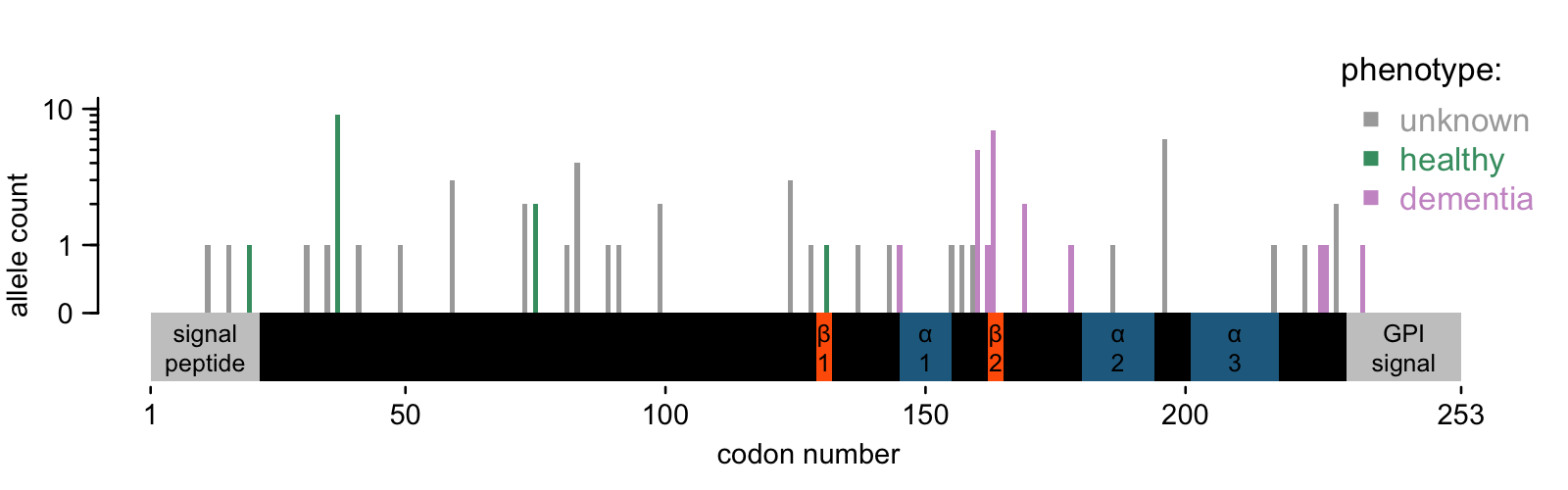
Here’s what the map of PRNP PTVs looks like today:
The 33 N-terminal variants are no surprise. We saw them in about 1 in 18,000 people in gnomAD v2, and we see them in 1 in 25,000 people in gnomAD v4 — quite close. All the conclusions from 2020 still stand. They are not constrained, consistent with having no phenotypic effect in the heterozygous state. And given their allele frequency, we wouldn’t expect to see homozygotes in an outbred population until we’ve sequenced a couple billion people. Don’t hold your breath.
But the C-terminal variants are surprising. If we count all 15 (possibly 17) in the same bucket, they are collectively wildly higher than we expected — approximately 1 in 50,000. That’s similar to the totality of genetic prion disease, and just as before, we’d further have to correct for the age distribution in gnomAD. And yet: in prion disease case cohorts, C-terminal PTVs are very, very rare. In our 2016 cohort, we had 10,460 patients, of whom 1895 had rare variants, and only 6 were PTVs — that’s 0.06% of all prion disease or 0.3% of genetic prion disease. Thus, to believe that all these PTVs are disease causing, and that gnomAD represents their true frequency in the population, would imply that the atypical prion disease associated with these variants is underdiagnosed by a factor of 300. I do think it’s probably underdiagnosed, but not by nearly such a factor. Likewise, sampling variance cannot begin to explain it, and the literature would suggest that C-terminal PTVs are highly penetrant, so I rather doubt a reduced penetrance explanation as well. And, probably because they are so highly penetrant, most literature reports on these variants are of single families — there are no known founder effects anywhere.
What’s going on then? Here, I think we are down to two possible explanations:
- Phenotypic enrichment. gnomAD v4 contains a lot of cohorts whose phenotypes could have accidentally enriched for pathogenic PRNP variants: two Alzheimer’s cohorts (ADSP and Kuopio), one ALS (ALSGen) and I count at least 14 different IBD cohorts. It would be of great interest to know whether the individuals harboring these variants come from the above cohorts.
- Positional effects. On the diagram above, I have denoted secondary structure elements in the structure of human PrP [Zahn 2000]: two beta sheets (β1 and β2) and 3 alpha helices (α1, α2, α3). You can see that the variants known to occur in prion cases cluster in a few places: before α1, between α1 & 2, and after α3. They leave some sizeable gaps where no PTV has ever been seen in a prion disease case, and the gnomAD v4 individuals partially fill in these gaps.
It inspires one to hypothesize that the exact position at which PrP is truncated — and, for frameshifts, what residues are added — might matter. Is this plausible? PrP is an incredibly well-studied protein, and the long list of structural mutants expressed in mice offers some support for the idea that exact position matters. In the late 1990s, a lot of labs were interested in finding the minimum amino acid sequence that could support prion replication. A 106-residue sequence (“PrP106”) that included a deletion from codon 142-177, spanning helix 1, was the winner. Deletions of helices 2 or 3 did not seem to support prion replication, even though deletion of everything from 145 onward does. It’s far from an exhaustive screen, and interstitial deletions are not the same thing as early stops, but it’s enough to suggest that the details matter. Even if all of these C-terminal PTVs leave intact the minimum sequence of PrP necessary for prion formation, some truncations might create a protein with secondary structure that inhibits misfolding, or with so little structure that it gets degraded before it has a chance. Still, all this is just a hypothesis, and one I could abandon quickly if it turned out that all 15 people with C-terminal truncating variants came from IBD or Alzheimer’s cohorts.
conclusions
Yes, sure enough: you sequence 6 times as many people, there’s a lot of new stuff to say about it. How much we’ll be able to follow up and solve the mystery of the C-terminal PTVs is an unknown. gnomAD was not designed to do genotype-first ascertainment and phenotyping, and it was only through incredible good will that we were able to do it on a very small scale in 2016 and 2020. Now the scale is larger and the data contributors and analysts busier. Still, I’m going to ask around and see what’s possible. If not now, someday, I hope we’ll get some answers.

About Eric Vallabh Minikel
Eric Vallabh Minikel is on a lifelong quest to prevent prion disease. He is a scientist based at the Broad Institute of MIT and Harvard.